Interpretable deep convolutional model for nonlinear multivariate time series in complex systems

Davor Horvatic; Domjan Baric

REVIEW 4 major objections 6 minor 29 references

Interpretable deep convolutional model for nonlinear multivariate time series in complex systems

T0 review · 4 major / 6 minor · reviewed 2026-08-10 · deepseek-v4-flash

Challenge this review Re-run · record.json Download PDF Read on arXiv ↗ Review JSON

Pith's one-line read DCIts claims a deep forecaster can output the exact coefficients of the equations generating a time series.

desk verdict A genuinely interpretable forecasting architecture with strong empirical coefficient recovery on synthetic benchmarks; the equation-reconstruction claim needs a scope limitation, but the paper deserves serious review. read the letter →

arxiv 2501.04339 v2 pith:GWSS2MGD submitted 2025-01-08 stat.ML cs.LGphysics.app-ph

Domjan Baric , Davor Horvatic This is my paper · ORCID

classification stat.MLcs.LGphysics.app-ph

keywords multivariatetimeseriesforecastinginterpretabledeeplearningmodelinterpretabilitymechanistictransitiontensorconvolutionalneuralnetworkhigher-ordertermscausaldiscovery

verification ladder T0 review T1 audit T2 compute T3 formal

The pith

A machine-rendered reading of the paper's core claim, the machinery that carries it, and where it could break.

The reading

DCIts is a deep convolutional forecaster for multivariate time series whose output includes, for every prediction window, a per-sample transition tensor $\alpha$ that says which source series, at which lags, with what sign and magnitude, drive each target series. The paper argues that on synthetic benchmarks with known generating equations, this tensor equals the ground-truth coefficient matrices to several decimal places, so DCIts is not just forecasting but reconstructing the equations that produced the data. It reports forecasting error equal to or better than the IMV-LSTM baseline while providing local interpretability for every sample. The point of the paper is that interpretability can be built into a deep forecaster as a factorization of its computations, with prediction accuracy acting as a faithfulness constraint.

What carries the argument

The load-bearing object is the transition tensor $\alpha \in \mathbb{R}^{N \times N \times L}$, whose entry $\alpha_{n,i,j}$ is the coefficient for how series $i$ at lag $j$ contributes to series $n$'s next value. DCIts computes $\alpha$ as the Hadamard (elementwise) product of two tensors produced by the same convolutional backbone: the Focuser $F = \sigma_T(H)$, a temperature-dependent sigmoid mask selecting relevant source-series and lag pairs, and the Modeler $C = W_H H + b_H$, an unconstrained linear coefficient map that can be negative and thus captures anti-correlation. The prediction is $X_{n,t+1} = \sum_{i,j} ((C \circ F) \diamondsuit Q_t)_{n,i,j}$, where $\diamondsuit$ denotes elementwise multiplication with broadcasting over the window $Q_t$. The extended version adds parallel Focuser and Modeler branches for the bias term ($p=0$) and for elementwise polynomial powers of the window ($p \ge 1$), giving order-resolved coefficients $\alpha^{(p)} = C^{(p)} \circ F^{(p)}$.

What would settle it

Run the same protocol on a dataset in which an unobserved variable drives both an observed cause and its effect, so the observed lags do not close the system; if DCIts still reports a stable nonzero $\alpha$ for the spurious link, the identity between $\alpha$ and the causal coefficients fails. A second, already-present check is Dataset 8's high-bias regime, where the paper reports a bias near 0.196 and a lag-one coefficient near 0.49 instead of the generating bias 0.7 and zero coefficients; a reader can rerun that experiment and look for the same miss.

Watch

Extended reading notes

Core claim

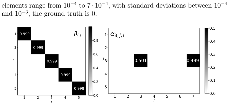
The paper's central claim is that the transition operator of a multivariate time series can be learned explicitly as $\alpha = C \circ F$, the Hadamard product of a Focuser mask $F$ and a Modeler coefficient tensor $C$, and that this $\alpha$ recovers the actual coefficients of the data-generating process. On a VAR(2) example the model returns entries such as $0.40 \pm 10^{-5}$ against ground truth $0.40$; on the autoregressive Dataset 2 it returns diagonal $\beta$ values near one against an identity ground truth; on the cross-correlated Dataset 4 it returns $\alpha_{1,2,2} = 0.396 \pm 0.004$ against the generating $2/5$; on Dataset 7 it recovers negative interactions such as $\alpha_{2,1,2} = -0.94 \pm 0.04$ against $-1$; and on the cubic process it recovers both linear and cubic coefficients with the correct sign and order while setting all quadratic terms to zero. Extended DCIts also detects regime-dependent dynamics in Dataset 8, where the learned coefficients split into bimodal distributions matching the switching ground truth, though the model misses the bias shift in the high regime.

Load-bearing premise

The data are assumed to be generated exactly by a finite-order polynomial (or linear) function of the observed lags of the observed series, with no unobserved confounders, and the forecasting loss is assumed to have a unique minimum at which the fitted coefficients equal the causal ones.

Editorial extensions

If this is right

From the learned $\alpha$ a user can read off the generating equations directly, as demonstrated by the VAR(2) reconstruction where all matrix entries match their ground-truth values to roughly $10^{-4}$ or better.
Per-sample $\alpha$ lets the model separate different regimes in one dataset: in Dataset 8 the coefficients $\alpha_{2,1,5}$ and $\alpha_{2,4,2}$ form bimodal distributions centered at the two switching ground truths.
The significance pattern of $\alpha$ also identifies the maximum relevant lag, so the window size can be chosen as the smallest lag with significant coefficients, as shown for Datasets 2, 4, and 7.
Higher-order branches recover the true polynomial order of the generator: on the cubic process the model finds the linear and cubic terms, finds no quadratic terms, and classifies the third series as purely linear.
Interpretability does not cost accuracy: DCIts reports equal or lower mean squared error than the IMV-LSTM baseline on all eight datasets in the paper.

Reading between the lines

Editorial extensions of the paper, not claims the author makes directly.

If the identity between $\alpha$ and the generating coefficients holds beyond polynomial synthetic systems, DCIts would give empirical researchers a signed, lag-resolved local causality map that current feature-importance methods do not provide.
The Dataset 8 bias miss suggests the factorization is not unique when a constant shift can be explained either by the bias branch or by a spurious lag coefficient; a diagnostic extension would be to compare $\alpha$ across multiple optima of the forecasting loss.
The order-resolved higher-order branches could double as a misspecification test: on non-polynomial dynamics the higher-order coefficients should scatter across samples instead of stabilizing, signaling that the interpretable polynomial form is not the right generator.

Share X Bluesky LinkedIn Reddit HN

Editorial analysis

A structured set of objections, weighed in public.

Desk editor's note, referee report, and a circularity audit.

Desk Editor's Note

read the letter

Domjan and Horvatic have built something real. The DCIts architecture—a Focuser that masks irrelevant lags and series, a linear Modeler that assigns signed coefficients, and a Hadamard product forming a per-sample transition tensor—is a clean, sensible design. The best evidence is the coefficient recovery: on the synthetic benchmarks, the learned α values match ground-truth matrices to 1e-3 or better, with tiny standard deviations across runs. That is not circular: the model is trained only on forecasting error, the ground-truth coefficients are external, and the data are generated from known equations. The higher-order extension and the bias term are straightforward but useful, and the GitHub release makes the work reproducible.

The soft spots are real but manageable. First, Eq. (4) has an index error: it multiplies by Q_{n,j} rather than Q_{i,j}. This is almost certainly a typo, but as written it obscures the model definition and should be fixed. Second, the 'statistically significant' language in Section 3.3 is never defined—no test, threshold, or procedure is given. Third, the loss function (MSE vs MAE) appears to be chosen after looking at results for some datasets; the paper should at least state this was a model selection decision, not a post hoc justification. Fourth, the benchmarks are the authors' own prior work; that is not a flaw by itself, but it means the evidence is narrower than a fully independent evaluation.

The load-bearing issue is identifiability. The paper claims the learned α reproduce the generating equations. But the forecasting loss constrains only the product C◦F, and C and F are unregularized outputs of a flexible network. Nothing in the architecture guarantees that the optimization's solution equals the true coefficients; the close matches on the benchmarks are encouraging but not a theorem. The authors do acknowledge the Dataset 8 failure—the model misses the bias shift and substitutes a spurious α instead—which is exactly the kind of failure this concern predicts. The paper should either provide an identifiability argument or explicitly scope the interpretability claim to cases where the data-generating process is within the model class and the optimization converges to the relevant solution.

For whom: applied researchers who want per-sample, signed, lag-resolved interaction structure from multivariate time series, and who are willing to treat the recovery as empirical rather than guaranteed. The paper deserves a serious referee, and with the notation fixed, the significance test described, and the identifiability limitation stated, it would be a solid contribution. I'd send it to review.

Referee Report

4 major / 6 minor

Summary. DCIts is an interpretable deep architecture for multivariate time series forecasting that factorizes the learned transition operator into a Focuser (a temperature-sigmoid mask) and a Modeler (an unconstrained coefficient tensor), yielding a per-sample transition tensor α = C ∘ F. The paper claims that α reproduces the ground-truth generating coefficients on synthetic benchmarks—so that forecasting accuracy certifies interpretability—and that the architecture extends to bias and polynomial higher-order terms. Forecasting performance is compared with IMV-LSTM on eight synthetic datasets, with additional experiments on a cubic map and on window-size selection.

Significance. If the reconstruction claim can be guaranteed or appropriately scoped, DCIts is a useful addition to interpretable time-series modeling: it provides per-sample, signed, lag-resolved coefficients; supports order-resolved polynomial extensions; is benchmarked on eight controlled datasets; reports variance over five runs; and ships open-source code. Close numerical matches to ground truth (e.g., the VAR(2) coefficients and the cubic-map terms) are genuinely encouraging. However, the central claim that α recovers the underlying equations currently rests on an unproven identifiability assumption, and the paper's own Dataset 8 bias-shift result contradicts the claim in one setting. The limitations paragraph in Section 4 does not discuss this core assumption, only computational cost and real-world noise. The paper needs either an identifiability proof under explicit assumptions or a formal narrowing of the interpretability claim.

major comments (4)

[2.1, Eq. (4)] Equation (4) defines (α♢Qt)n,i,j = αn,i,j × Qn,j, but given the stated meaning of αn,i,j as the effect of the ith series at lag j on the nth target, the multiplication should be with Qi,j, not Qn,j. As written, the equation contracts the wrong index and is inconsistent with the tensor shapes in Eq. (3) and Eq. (10). Please correct the typo or, if the indexing is intentional, explain how the additional n-dependence arises.
[2.1, 2.2, 3.3.4] The interpretability claim is not identified by the forecasting objective. The loss depends on α only through the prediction (C∘F)♢Qt, so for any sample Qt one can add a per-sample tensor Bt that is annihilated by the contracted product with Qt without changing the loss. Since F and C are per-sample, unregularized outputs of a flexible network, many coefficient tensors attain the same loss. The paper nevertheless concludes in Section 3.3.4 and Section 4 that α reconstructs the generating equations. The Dataset 8 bias result in Section 3.3.4 (b1 = 0.196 ± 0.004 for both regimes, ground truth 0.2 and 0.7) shows concretely that a low-loss solution need not match the generator. Please add either a formal identifiability proof under stated assumptions (e.g., uniqueness of the minimizer within the factorized family) or an explicit limitation stating that α is only an interpretation of the fitted model, and that equality to the data-generating coefficients is an empirical property demonstrated on the synthetic benchmarks, not a guaranteed consequence of the method.
[3.2, Figure 8] The phrase 'statistically significantly different from zero' is never defined. No test statistic, null distribution, threshold, or multiple-comparison procedure is given. This filter is load-bearing because it is used to conclude that all α1,j,l with l > 5 are zero for Dataset 7. Please specify the exact significance test used, how the null distribution was obtained (e.g., across runs, across samples), and how multiple testing over (i,j,l) was handled, or remove the significance wording and report raw coefficient distributions instead.
[3.3, 3.3.2] The choice of loss function for the interpretability results appears to be made post hoc. The paper states that results use MAE 'unless stated otherwise,' and Dataset 4 is singled out as a case where 'MAE behaves better with respect to MSE.' If the loss was selected after inspecting interpretability performance on the test set, the reported faithfulness is optimistically biased. Please clarify whether the loss was selected on a validation set, describe the pre-specified selection rule, or report results for both MSE and MAE on all datasets.

minor comments (6)

[2.1, Eq. (9)] The sigmoid formula σT(x) = 1/(1 − e^{−x/T}) appears to have an incorrect sign in the denominator; the standard temperature-sigmoid is 1/(1 + e^{−x/T}). As written, the formula has a singularity at x = 0 and outputs outside (0,1).
[2.4, Figure 3 and Eq. (15)] The notation for the p = 0 term is under-specified: the product ⃝0 is defined as the identity matrix I, but the dimensions of C0, F0, and the broadcasting rule for (C0∘F0)♢I are not stated. Please clarify how the bias term is represented for each target series n.
[3.1, Table 1 and Figure 5] The text alternates between 'DCIts' and 'DCITs'; please standardize the acronym throughout, including in table and figure captions.
[Abstract and Introduction] The claim that the model 'matches or often surpasses existing interpretability methods' is supported only by a comparison with IMV-LSTM. Adding at least one more recent interpretable baseline or softening the claim would make the statement proportionate.
[2.1] The statement 'we did extensive analysis on the influence of temperature' is not accompanied by any results. Either report a temperature-sensitivity experiment (e.g., in supplementary material) or remove the claim.
[Appendix A, Dataset 8] The Appendix text says 'bhigh and bhigh switch, based on a persistence duration' — the duplicated 'bhigh' appears to be a typo; it should read 'blow and bhigh switch.'

Circularity Check

0 steps flagged · score 0.0 of 10

No significant circularity: coefficient recovery is evaluated against externally specified ground truth and can fail (Dataset 8).

full rationale

The central interpretability claim is that the learned per-sample tensor α = C ◦ F (Eq. 12) reproduces the coefficients of the data-generating process. The chain is not circular: the model is optimized only on the forecasting loss (MSE/MAE), and the ground-truth coefficients used for evaluation (Appendix A, the VAR(2) process, and the Cubic process) are specified independently and are never given to the model. The paper quotes specific recovered values with standard deviations and also reports a failure on the Dataset 8 bias shift (Section 3.3.4), which demonstrates that the evaluation is falsifiable and not forced by construction. The benchmarks and the IMV-LSTM baseline come from the authors' prior work, but this is ordinary self-citation: the datasets' ground truth is externally defined by the generating equations, and the DCIts training objective does not include those coefficients. The definition α = C ◦ F is a modeling ansatz, not a hidden reuse of the target result. The statement about zero α(2) values in Section 3.4 could be trivial if no quadratic branch were instantiated, but the text indicates higher-order branches were included and the claim is peripheral; it does not affect the central coefficient-reconstruction result. Overall, the derivation is self-contained and the main interpretability claim has independent empirical content.

Assumptions & free parameters 6 free parameters · 4 assumptions · 0 invented entities

The model itself contains thousands of learnable weights, which are not listed here. The listed items are hyperparameters and assumptions that the central interpretability claim depends on. The biggest epistemic risk is the untested assumption that the observed window contains all causal variables and that the generating process lies in the polynomial model class.

free parameters (6)

Temperature T of sigmoid in Focuser = 1
Set to 1 by hand; paper says extensive analysis showed no benefit from changing, but no results shown.
Window size L = 10 for comparison, per-dataset optimal 5-9
Chosen by validation loss; used for direct comparison to IMV-LSTM.
Loss function = MAE (default), MSE for some
Chosen per dataset based on validation and interpretability behavior; potential post hoc selection.
Number of convolutional layers = 7
Selected after exhaustive subset search; the paper does not report the per-layer filter counts.
Number of fully connected layers HN = 3
Selected from 1-5 via validation; no detailed criterion.
Number of runs R = 5
Used for averaging and statistical significance, chosen by convention.

assumptions (4)

domain assumption The multivariate time series is generated by a deterministic function of its past L lags plus noise (Markov-order L).
Equation (1) assumes X_{t+1} = αQ_t; the model cannot represent regimes beyond the chosen L or unobserved external drivers.
domain assumption The true generating function can be represented by a finite polynomial expansion in the observed variables (linear or higher-order) with finite order.
The interpretability claim equates learned α(p) coefficients with ground truth generating coefficients; this is only meaningful if the generator is in the model class. Section 2.4 introduces higher-order terms to cover polynomial nonlinearities, but arbitrary nonlinearities (e.g., tanh in Dataset 6) are only approximated locally.
domain assumption The training procedure converges to a global optimum that yields the causal coefficients rather than an alternative local representation with equal loss.
No identifiability or convergence guarantee is provided; the paper relies on empirical repetition and a fixed seed for stability. If multiple equivalent coefficient sets exist, the interpretation may be arbitrary.
domain assumption No unobserved confounders affect the target series beyond the N observed series.
The transition tensor has support only on observed series; unobserved common causes would appear as cross-series coefficients and be misattributed.

how reviews work

0 comments

Cite this review

Pith. "Pith review of Interpretable deep convolutional model for nonlinear multivariate time series in complex systems." pith.science (2026). https://pith.science/paper/GWSS2MGD

@misc{pith2026250104339,
  author       = {Pith},
  title        = {Pith review of: Interpretable deep convolutional model for nonlinear multivariate time series in complex systems},
  year         = {2026},
  howpublished = {\url{https://pith.science/paper/GWSS2MGD}},
  note         = {Machine review of arXiv:2501.04339}
}

read the original abstract

We introduce the Deep Convolutional Interpreter for Time Series (DCIts), a deep-learning architecture for nonlinear multivariate time series that provides sample-specific, locally interpretable descriptions of the underlying interaction structure. Unlike standard black-box forecasters, DCIts learns a time- and lag-dependent transition tensor explicitly factorized into two components: a Focuser, which selects relevant source series and time lags via a sparse masking mechanism, and a Modeler, which assigns signed coefficients to these selected interactions. This decomposition yields a local lag-adjacency structure and signed source-lag contributions for every forecast instance, enabling direct inspection of effective connectivity; when higher-order branches are activated, the same framework yields order-resolved elementwise polynomial contributions. Architecturally, DCIts uses a diverse bank of convolutional filters to capture temporal and cross-variable dependencies, which are mapped through a bottleneck network to the transition tensor. On controlled benchmark datasets with a known interaction structure, we demonstrate that DCIts achieves competitive forecasting error relative to a strong interpretable baseline while recovering stable, signed, lag-resolved interaction patterns. The framework thus prioritizes intrinsic interpretability, using forecasting accuracy as a faithfulness constraint rather than the sole objective.

Figures

Figures reproduced from arXiv: 2501.04339 by the authors.

**Figure 2.** The left figure illustrates the architecture of the Focuser, while the right figure [PITH_FULL_IMAGE:figures/full_fig_p007_2.png] view at source ↗

**Figure 3.** The architecture of the extended DCIts model incorporates bias and higher [PITH_FULL_IMAGE:figures/full_fig_p014_3.png] view at source ↗

Figures from the paper (12 more)

**Figure 4.** Figure 4: The stability of prediction performance by dataset is assessed by plotting the [PITH_FULL_IMAGE:figures/full_fig_p017_4.png]

**Figure 5.** Figure 5: The left figure illustrates how the stability of prediction performance for a specific [PITH_FULL_IMAGE:figures/full_fig_p018_5.png]

**Figure 6.** Figure 6: Parallel coordinates plot of evaluated models within Performance-Explainability [PITH_FULL_IMAGE:figures/full_fig_p019_6.png]

**Figure 7.** Figure 7: Impact of window size on loss. On the x-axis we plot window size, on the y-axis, [PITH_FULL_IMAGE:figures/full_fig_p020_7.png]

**Figure 8.** Figure 8: Statistically significant α1,j,l values for Dataset 7 with L = 7 and R = 5. All α1,j,l elements with l > 5 are correctly identified as zero. marking datasets, we first demonstrate the strength of the DCIts architecture using a simple second-order vector autoregressive …

**Figure 9.** Figure 9: In the left panel, the β coefficients estimated by DCIts for Dataset 2 are shown. The y-axis corresponds to the target series index, and the x-axis corresponds to the source time series. Since this dataset consists solely of autoregressive time series with no interact…

**Figure 10.** Figure 10: Mean α values for Dataset 4, obtained using MAE as the loss functions by Algorithm 1 match ground truth values. The y-axis corresponds to the source time series index (j), and the x-axis represents the time lag (l). In Datasets 5 and 6, each time series is generated b…

**Figure 11.** Figure 11: Mean β values estimated by DCIts using MSE (left panel) and α4,j,l values (right panel) for Dataset 5. The ground truth is given by βi,1 = 1 for all i, with all other β values being zero. Each time series in this dataset depends solely on X1,t, and DCIts correctly ide…

**Figure 12.** Figure 12: presents the results for the α2,j,l and α4,j,l coefficients: α gt 2,1,2 = −1, α2,1,2 = (−0.94 ± 0.04); α gt 4,3,4 = −2/7 ≈ −0.286, α4,3,4 = (−0.27 ± 0.02); α gt 4,5,1 = −5/7 ≈ −0.714, α4,5,1 = (−0.71±0.01). DCIts successfully identified the correct lags and accurately…

**Figure 13.** Figure 13: Histograms for α2,1,5 (left) and α2,4,2 (right). Both distributions are bimodal (elements are either close to zero or to ground truth), indicating that DCIts successfully detected the two different dynamics in this dataset. F2,j,l, i.e., the p = 1 focuser values for X…

**Figure 14.** Figure 14: Mean focuser F2,j,l values for X1,t−5 ≤ 0.5 (left panel) and X1,t−5 > 0.5 (right panel) from the DCIts model for Dataset 8. The y-axis corresponds to the source time series j, and the x-axis corresponds to the lag l. The focuser correctly identified the most important…

**Figure 15.** Figure 15: β˜ coefficients for linear and cubic terms learned by DCIts, and ground truth values for the Cubic process. DCIts learned correctly both linear and cubic terms, and it also learned that X3,t is just the linear combination of X1,t and X2,t which are both cubic maps. to…

Discussion (0). Continue with ORCID to comment.

Reference graph

Works this paper leans on

29 extracted references · 15 canonical work pages

[1]

Chen, C.-L

S.-A. Chen, C.-L. Li, S. O. Arik, N. C. Yoder, T. Pfister, TSMixer: An all-MLP architecture for time series forecast-ing, Transactions on Machine Learning Research (2023). URL: https://openreview.net/ forum?id=wbpxTuXgm0

work page 2023
[2]

Bari´ c, P

D. Bari´ c, P. Fumi´ c, D. Horvati´ c, T. Lipic, Benchmarking attention- based interpretability of deep learning in multivariate time series predic- tions, Entropy 23 (2021). URL: https://www.mdpi.com/1099-4300/ 23/2/143

work page 2021
[3]

A Performance-Explainability Framework to Benchmark Machine Learning Methods: Application to Multivariate Time Series Classifiers

K. Fauvel, V. Masson, ´E. Fromont, A performance-explainability frame- work to benchmark machine learning methods: Application to multivari- ate time series classifiers, arXiv preprint arXiv:2005.14501 (2020)

work page Pith review arXiv 2020
[4]

T. Guo, T. Lin, N. Antulov-Fantulin, Exploring interpretable lstm neu- ral networks over multi-variable data, 2019. arXiv:1905.12034

arXiv 2019
[5]

Ozyegen, I

O. Ozyegen, I. Ilic, M. Cevik, Evaluation of interpretability methods for multivariate time series forecasting, Applied Intelligence 52 (2022) 4727–

work page 2022
[6]

Schlegel, D

U. Schlegel, D. V. Lam, D. A. Keim, D. Seebacher, TS-MULE: lo- cal interpretable model-agnostic explanations for time series forecast models, CoRR abs/2109.08438 (2021). URL: https://arxiv.org/abs/ 2109.08438. arXiv:2109.08438

arXiv 2021
[7]

S. M. Lundberg, S.-I. Lee, A unified approach to interpreting model predictions, in: Advances in neural information processing systems, 2017, pp. 4765–4774

work page 2017
[8]

An Empirical Study of Explainable AI Techniques on Deep Learning Models For Time Series Tasks

U. Schlegel, D. Oelke, D. A. Keim, M. El-Assady, An empirical study of explainable AI techniques on deep learning models for time series tasks, CoRR abs/2012.04344 (2020). URL: https://arxiv.org/abs/ 2012.04344. arXiv:2012.04344

work page Pith review arXiv 2020

Show all 29 references

[9]

Gangopadhyay, S

T. Gangopadhyay, S. Y. Tan, Z. Jiang, R. Meng, S. Sarkar, Spatiotem- poral attention for multivariate time series prediction and interpreta- tion, CoRR abs/2008.04882 (2020). URL: https://arxiv.org/abs/ 2008.04882. arXiv:2008.04882. 34

2020 arXiv
[10]

A.-D. Pham, A. Kuestenmacher, P. G. Ploeger, Tsem: Temporally- weighted spatiotemporal explainable neural network for multivariate time series, in: K. Arai (Ed.), Advances in Information and Communi- cation, Springer Nature Switzerland, Cham, 2023, pp. 183–204

2023
[11]

B. Wu, L. Wang, Y.-R. Zeng, Interpretable tourism demand fore- casting with temporal fusion transformers amid covid-19, Applied In- telligence 53 (2023) 14493–14514. URL: https://doi.org/10.1007/ s10489-022-04254-0 . doi:10.1007/s10489-022-04254-0

2023 doi
[12]

Pantiskas, K

L. Pantiskas, K. Verstoep, H. Bal, Interpretable multivariate time series forecasting with temporal attention convolutional neural networks, in: 2020 IEEE Symposium Series on Computational Intelligence (SSCI), 2020, pp. 1687–1694. doi: 10.1109/SSCI47803.2020.9308570

2020
[13]

S. Feng, C. Miao, K. Xu, J. Wu, P. Wu, Y. Zhang, P. Zhao, Multi- scale attention flow for probabilistic time series forecasting, 2023. arXiv:2205.07493

2023 arXiv
[14]

Gandin, A

I. Gandin, A. Scagnetto, S. Romani, G. Barbati, Interpretability of time-series deep learning models: A study in cardiovascular patients admitted to intensive care unit, Journal of Biomedical Informatics 121 (2021) 103876. URL: https://www.sciencedirect.com/science/ article/pi...

2021
[15]

S. Jain, B. C. Wallace, Attention is not explanation, CoRR abs/1902.10186 (2019). URL: http://arxiv.org/abs/1902.10186. arXiv:1902.10186

2019 arXiv
[16]

Wiegreffe, Y

S. Wiegreffe, Y. Pinter, Attention is not not explanation, CoRR abs/1908.04626 (2019). URL: http://arxiv.org/abs/1908.04626. arXiv:1908.04626

2019 arXiv
[17]

B. N. Oreshkin, D. Carpov, N. Chapados, Y. Bengio, N-BEATS: neural basis expansion analysis for interpretable time series forecast- ing, CoRR abs/1905.10437 (2019). URL: http://arxiv.org/abs/ 1905.10437. arXiv:1905.10437

2019 arXiv
[18]

Rasul, A

K. Rasul, A. Sheikh, I. Schuster, U. Bergmann, R. Vollgraf, Multi- variate probabilistic time series forecasting via conditioned normalizing 35 flows, CoRR abs/2002.06103 (2020). URL: https://arxiv.org/abs/ 2002.06103. arXiv:2002.06103

2020 arXiv
[19]

Munkhdalai, T

L. Munkhdalai, T. Munkhdalai, V.-H. Pham, M. Li, K. H. Ryu, N. Theera-Umpon, Recurrent neural network-augmented locally adaptive interpretable regression for multivariate time-series forecast- ing, IEEE Access 10 (2022) 11871–11885. doi: 10.1109/ACCESS.2022. 3145951

2022 doi
[20]

Panja, T

M. Panja, T. Chakraborty, U. Kumar, A. Hadid, Probabilistic autore- gressive neural networks for accurate long-range forecasting, in: B. Luo, L. Cheng, Z.-G. Wu, H. Li, C. Li (Eds.), Neural Information Processing, Springer Nature Singapore, Singapore, 2024, pp. 457–477

2024
[21]

Fauvel, T

K. Fauvel, T. Lin, V. Masson, ´E. Fromont, A. Termier, XCM: an ex- plainable convolutional neural network for multivariate time series clas- sification, CoRR abs/2009.04796 (2020). URL: https://arxiv.org/ abs/2009.04796. arXiv:2009.04796

2020 arXiv
[22]

Assaf, A

R. Assaf, A. Schumann, Explainable deep neural networks for multi- variate time series predictions., in: IJCAI, 2019, pp. 6488–6490

2019
[23]

J. Wang, Z. Wang, J. Li, J. Wu, Multilevel wavelet decom- position network for interpretable time series analysis, CoRR abs/1806.08946 (2018). URL: http://arxiv.org/abs/1806.08946. arXiv:1806.08946

2018 arXiv
[24]

Castro, P

M. Castro, P. R. Mendes J´ unior, A. Soriano-Vargas, R. de Oliveira Wer- neck, M. Moreira Gon¸ calves, L. Lusquino Filho, R. Moura, M. Zampieri, O. Linares, V. Ferreira, A. Ferreira, A. Dav´ olio, D. Schiozer, A. Rocha, Time series causal relationships discovery through featur...

2023 doi
[25]

X. Dang, S. Y. Shah, P. Zerfos, seq2graph: Discovering dynamic dependencies from multivariate time series with multi-level attention, CoRR abs/1812.04448 (2018). URL: http://arxiv.org/abs/1812. 04448. arXiv:1812.04448. 36

2018 arXiv
[26]

Y. Qin, D. Song, H. Chen, W. Cheng, G. Jiang, G. W. Cottrell, A dual-stage attention-based recurrent neural network for time series pre- diction, CoRR abs/1704.02971 (2017). URL: http://arxiv.org/abs/ 1704.02971. arXiv:1704.02971

2017 arXiv
[27]

Bari´ c, D

D. Bari´ c, D. Horvati´ c, dcits, https://github.com/hc-xai/dcits,
[2024]

Maintained by the authors, Accessed: January 6th 2025. 37

2025
[4743]

URL: https://doi.org/10.1007/s10489-021-02662-2 . doi:10. 1007/s10489-021-02662-2

doi

Pith tools

Reviewed August 10, 2026 · model on record in the stance chip above.

[1] [1]

Chen, C.-L

S.-A. Chen, C.-L. Li, S. O. Arik, N. C. Yoder, T. Pfister, TSMixer: An all-MLP architecture for time series forecast-ing, Transactions on Machine Learning Research (2023). URL: https://openreview.net/ forum?id=wbpxTuXgm0

work page 2023

[2] [2]

Bari´ c, P

D. Bari´ c, P. Fumi´ c, D. Horvati´ c, T. Lipic, Benchmarking attention- based interpretability of deep learning in multivariate time series predic- tions, Entropy 23 (2021). URL: https://www.mdpi.com/1099-4300/ 23/2/143

work page 2021

[3] [3]

A Performance-Explainability Framework to Benchmark Machine Learning Methods: Application to Multivariate Time Series Classifiers

K. Fauvel, V. Masson, ´E. Fromont, A performance-explainability frame- work to benchmark machine learning methods: Application to multivari- ate time series classifiers, arXiv preprint arXiv:2005.14501 (2020)

work page Pith review arXiv 2020

[4] [4]

T. Guo, T. Lin, N. Antulov-Fantulin, Exploring interpretable lstm neu- ral networks over multi-variable data, 2019. arXiv:1905.12034

arXiv 2019

[5] [5]

Ozyegen, I

O. Ozyegen, I. Ilic, M. Cevik, Evaluation of interpretability methods for multivariate time series forecasting, Applied Intelligence 52 (2022) 4727–

work page 2022

[6] [6]

Schlegel, D

U. Schlegel, D. V. Lam, D. A. Keim, D. Seebacher, TS-MULE: lo- cal interpretable model-agnostic explanations for time series forecast models, CoRR abs/2109.08438 (2021). URL: https://arxiv.org/abs/ 2109.08438. arXiv:2109.08438

arXiv 2021

[7] [7]

S. M. Lundberg, S.-I. Lee, A unified approach to interpreting model predictions, in: Advances in neural information processing systems, 2017, pp. 4765–4774

work page 2017

[8] [8]

An Empirical Study of Explainable AI Techniques on Deep Learning Models For Time Series Tasks

U. Schlegel, D. Oelke, D. A. Keim, M. El-Assady, An empirical study of explainable AI techniques on deep learning models for time series tasks, CoRR abs/2012.04344 (2020). URL: https://arxiv.org/abs/ 2012.04344. arXiv:2012.04344

work page Pith review arXiv 2020