REVIEW 1 major objections 4 minor 15 references
Gibbs sampling for game-theoretic modeling of private network upgrades with distributed generation
T0 review · 1 major / 4 minor · reviewed 2026-08-14 · deepseek-v4-flash
Pith's one-line read The paper shows that Gibbs sampling can supply the stochastic scenarios needed to compute the Stackelberg equilibrium of a private network upgrade game, and that the resulting optimal capacities are stable to within about 10 MW on a real…
desk verdict A plausible integration of Gibbs sampling with a Stackelberg investment game, undermined by a sign error in the curtailment pseudocode that, if present in the code, inverts the central cost in the profit equations. read the letter →
The pith
A machine-rendered reading of the paper's core claim, the machinery that carries it, and where it could break.
The reading
What carries the argument
The load-bearing object is the Gibbs sampler in Algorithm 1, which cycles through the three variables $(w_1, w_2, P_D)$ by sampling each wind speed from the empirical conditional distribution of the other site's wind speed and then sampling demand from the empirical conditional distribution given the average wind speed, with a burn-in of 20% of samples to erase dependence on the starting state. This generates synthetic wind and demand series that are passed to Algorithm 2, which uses a sigmoid power curve to convert wind speed to per-unit power and computes total generation and curtailment for every pair of rated capacities. Algorithm 3 then evaluates the two profit functions for those generation and curtailment totals and finds the Stackelberg equilibrium by backward induction. The machinery works because the Gibbs chain's sample mean converges to the historical mean as the sample size grows, which the paper verifies by increasing $n$ and $N$ and tracking the maximum error from the historical mean.
What would settle it
Hold out a period of historical demand not used in building the conditional table, sample demand from $G(P_D \mid (w_1+w_2)/2)$ for the same period's wind speeds, and compare the sampled distribution with the actual held-out demand. If the two differ substantially in seasonal shape, autocorrelation, or tail behaviour, the equilibrium capacities are not trustworthy. A second check is to rerun the Stackelberg search with an alternative demand model, such as a temperature-driven or autoregressive model, and see whether the equilibrium capacities move outside the reported 10 MW range.
Extended reading notes
Core claim
The central claim is that Markov chain Monte Carlo, specifically Gibbs sampling, makes the equilibrium computation tractable by replacing an unknown analytic joint distribution with empirical conditional distributions built from data. For each player's wind speed, the sampler draws a new value conditional on the other player's current value, then draws demand conditional on the average of the two wind speeds; after discarding a burn-in period, the resulting chain approximates the historic joint distribution. These synthetic hourly observations feed a full enumeration of capacity pairs, from which expected generation, curtailment, and profits are computed, and backward induction yields the leader's capacity $P^*_{N1}$ and the follower's best response $P^*_{N2}$. The paper reports that these equilibrium capacities show a 10 MW range across realisations and that, as generation costs or the transmission fee rise, total installed capacity falls, with the follower's cost having the larger leverage on both players' capacities.
Load-bearing premise
The load-bearing premise is that demand at the consumer node is fully captured by the empirical conditional distribution of historical demand given the average wind speed at the two wind-farm sites; if real demand responds mainly to temperature, season, or time of day rather than wind, the simulated curtailment and the resulting equilibrium capacities and profits will be off.
Editorial extensions
If this is right
- With a sufficiently large Gibbs sample (here $n = 50{,}000$ after burn-in), the simulated wind speeds and demand reproduce the historical means, so the method can generate large synthetic datasets even when historical records have gaps.
- The equilibrium capacities $(P^*_{N1}, P^*_{N2})$ can be recomputed for any set of cost parameters, so the model maps how generation costs and transmission fees shift who builds what.
- There is a minimum transmission fee, around £12/MWh or $p_T \approx 0.16 p_G$, below which the line investor cannot break even, and an upper bound above which local generators stop investing, giving a feasible regulatory range.
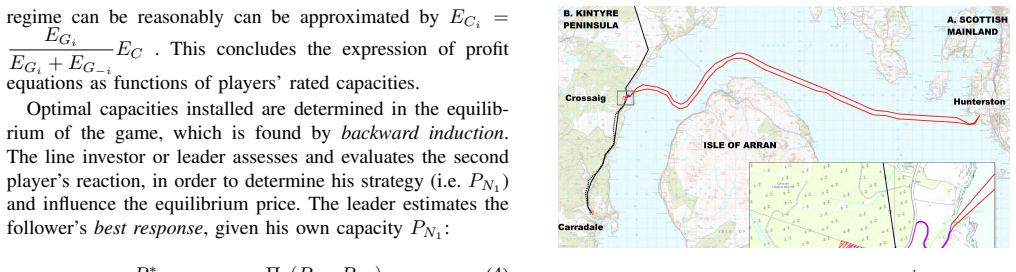
- Across 170 Monte Carlo realisations of the Kintyre–Hunterston case, equilibrium optimal capacities vary within a 10 MW band, suggesting that scenario-sampling uncertainty does not dominate the investment decision.
- Because the game is set up for any two-node system where demand and renewable generation are not co-located, the same pipeline applies to other constrained network upgrade problems with wind and demand data.
Reading between the lines
- A natural extension, not pursued in the paper, is multi-location sampling: pair each site's wind with a conditional distribution over all other sites, but the chain's mixing and convergence would need separate testing because sparse conditional bins multiply with dimension.
- The demand model $P_D \mid (w_1+w_2)/2$ is the fragile link. Replacing it with a demand model that includes seasonality, temperature, or time-of-day would be a direct stress test; if the equilibrium capacities move outside the reported 10 MW band, the current demand assumption is the cause.
- The reported 10 MW stability likely understates total uncertainty because the paper holds cost parameters, the power curve, and the demand conditional fixed across realisations; a full propagation of these uncertainties would widen the credible range.
- The comparative-statics result—total capacity falls as costs or fees rise—suggests a regulator can use this pipeline to set $p_T$ before construction, searching for the fee that keeps both players profitable while maximising installed renewable capacity.
Signed reviews
Editorial analysis
A structured set of objections, weighed in public.
Referee Report
Summary. The paper proposes a methodology that combines Gibbs sampling with a Stackelberg game model to determine optimal generation capacities for a private network upgrade. Wind speed and demand scenarios are generated from historical data via a Gibbs sampler, and these scenarios are used to compute expected generation, curtailment, and profits for a line investor (leader) and local generators (follower). The approach is applied to the Kintyre-Hunterston link in the UK, and the paper reports convergence diagnostics for the sampler and equilibrium capacities and profits across multiple realisations and cost scenarios.
Significance. If the methodology is sound, the paper offers a useful template for using MCMC scenario generation in game-theoretic investment models with stochastic renewable resources, which is a relevant problem for network planning. The authors provide a reasonably detailed description of the Gibbs sampler and report internal convergence checks (Tables I and II) that show the expected central-limit behavior for increasing sample size. However, the central algorithm contains a sign error in the curtailment calculation that directly affects the equilibrium results, and the conditional demand model is not validated. These issues must be resolved before the claims can be trusted.
major comments (1)
- [Algorithm 2, lines 7–12] The curtailment calculation has a sign error. With RD = PD - (PG1 + PG2), a curtailment event corresponds to RD < 0, but lines 11–12 compute PC1 = PG1 * RD / (PG1 + PG2) and PC2 = PG2 * RD / (PG1 + PG2), which are negative when generation exceeds demand. This reverses the sign of curtailment, so the terms (EGi - ECi) in Eqs. (1)–(2) exceed EGi, inflating revenues and distorting the best-response calculations. This is not a cosmetic typo: the published algorithm implements the opposite sign in exactly the state-space region that defines the game. If the reported results were produced by code matching the pseudocode, the equilibrium capacities and profits in Figs. 2–3 are not trustworthy; if the code used a corrected sign, the pseudocode omits a sign convention essential for reproducibility. The paper provides no clarification or erratum, so the central claim is not reproducible from the published algorithm.
minor comments (4)
- [Section II] The sentence 'curtailment expressions for each player under a “common access” regime can be reasonably can be approximated by ECi = EGi/(EGi + EG−i) EC' contains a duplicated phrase 'can be reasonably can be'; please revise to 'can be reasonably approximated by'.
- [References] Reference [3] lists 'IEEE 2012 PES ISGT Europe' but is dated 2016; either the conference year or the publication year is inconsistent, and the venue should be checked.
- [Tables I and II] In Table II, the maximum error (ME) for wind speed does not decrease as the number of realisations N increases (e.g., ME for w1 goes from 6.64% at N=100 to 9.87% at N=50,000). The text explains that WCI narrows, but the ME behavior is not discussed; please clarify whether ME is the deviation of the overall sample mean from the historic mean and why it does not improve with N.
- [Section IV.B, text after Table I] The text states 'µw1 = 12.1029, µw1 = 12.1950' for the historic means; the second symbol should likely be µw2. Please correct the notation.
Circularity Check
No significant circularity; the only near-circular step is the internal-consistency validation of the Gibbs sampler against the historic statistics used to build it.
-
fitted input called prediction
[Section IV-B, Tables I and II (validation of Gibbs sampler)]
"Columns represent the sample mean, standard deviation of the sample mean, width of the 95% confidence interval (WCI) and maximum error (ME) from mean of historic data, i.e. µw1 = 12.1029, µw1 = 12.1950 and µPD = 108.1830."
Algorithm 1 (lines 4-5, 9-11) builds the conditional distributions F(w1|w2), F(w2|w1), and G(PD|(w1+w2)/2) directly from the historic wind and demand data, so the historic means µw1, µw2, µPD are inputs to the sampler. Tables I and II then 'validate' the MCMC by checking that sample means converge to those same historic means. For an ergodic Markov chain, the sample mean converges to the stationary distribution, which is exactly the empirical joint distribution used to construct the conditionals; hence this check is guaranteed in the limit and is an internal-consistency test, not an independent prediction. It does not test the modeling assumption that demand depends only on average wind speed.
full rationale
The paper's derivation chain is otherwise self-contained. Wind and demand scenarios are generated by a Gibbs sampler whose conditional tables are empirical histograms of historic data; Algorithm 2 converts sampled wind speeds to power outputs and curtailment; Algorithm 3 computes profits and finds the Stackelberg equilibrium by explicit best-response optimization. The reported optimal capacities (P_N1*, P_N2*) are not fitted to the output or defined in terms of the result, so the central game-theoretic claim is not circular. Self-citations to [3] and [11] supply the profit and curtailment equations, but those equations are reproduced in the text and are not used as an unexamined uniqueness theorem or ansatz imported by citation. The skeptical observation about Algorithm 2's sign of curtailment when generation exceeds demand (RD < 0) is a potential correctness/reproducibility issue, not a circularity issue. The nonzero score reflects only the internal-consistency validation of the sampler, which compares the simulated means with the historic means used to construct the conditional distributions.
Assumptions & free parameters
free parameters (5)
- alpha (sigmoid slope of wind power curve) =
not reported
- beta (sigmoid midpoint of wind power curve) =
not reported
- CT (total line cost, investment plus O&M) =
not reported
- Capacity search grid (PNmax, step) =
500.5 MW, 0.5 MW
- MCMC tuning (n, N, burn-in) =
n=50,000, N=170, burn-in=10,000
assumptions (5)
- domain assumption The empirical conditional distribution tables built from 17 years of Met Office data, with sparse bins merged, represent the true joint wind speed distribution at both locations.
- domain assumption Demand at location A is drawn from the conditional distribution G(P_D | (w1+w2)/2), so wind speed is the only driver of demand variation.
- domain assumption Under common access, curtailed energy is apportioned to each player in proportion to its generation share, ECi = EGi/(EGi+EG-i) EC.
- domain assumption Both players maximize profit and the outcome is the subgame-perfect Stackelberg equilibrium found by backward induction.
- domain assumption Historic wind and demand statistics are stationary over the project lifetime, so sampling from past data represents future scenarios.
Cite this review
Pith. "Pith review of Gibbs sampling for game-theoretic modeling of private network upgrades with distributed generation." pith.science (2026). https://pith.science/paper/H5A37LZ5
@misc{pith2026190810862,
  author       = {Pith},
  title        = {Pith review of: Gibbs sampling for game-theoretic modeling of private network upgrades with distributed generation},
  year         = {2026},
  howpublished = {\url{https://pith.science/paper/H5A37LZ5}},
  note         = {Machine review of arXiv:1908.10862}
}
read the original abstract
Renewable energy is increasingly being curtailed, due to oversupply or network constraints. Curtailment can be partially avoided by smart grid management, but the long term solution is network reinforcement. Network upgrades, however, can be costly, so recent interest has focused on incentivising private investors to participate in network investments. In this paper, we study settings where a private renewable investor constructs a power line, but also provides access to other generators that pay a transmission fee. The decisions on optimal (and interdependent) renewable capacities built by investors, affect the resulting curtailment and profitability of projects, and can be formulated as a Stackelberg game. Optimal capacities rely jointly on stochastic variables, such as the renewable resource at project location. In this paper, we show how Markov chain Monte Carlo (MCMC) and Gibbs sampling techniques, can be used to generate observations from historic resource data and simulate multiple future scenarios. Finally, we validate and apply our game-theoretic formulation of the investment decision, to a real network upgrade problem in the UK.
Figures


Reference graph
Works this paper leans on
-
[11]
Game-theoretic modeling of curtailment rules and network investments with distributed generation,
M. Andoni, V . Robu, W.-G. Fr ¨uh, and D. Flynn, “Game-theoretic modeling of curtailment rules and network investments with distributed generation,” Applied Energy, vol. 201, pp. 174–187, 2017
work page 2017
-
[1]
FPP low carbon networks: Commercial solutions for active network management,
A. Laguna Estopier, E. Crosthwaite Eyre, S. Georgiopoulos, and C. Marantes, “FPP low carbon networks: Commercial solutions for active network management,” in CIRED, Stockholm, 2013
work page 2013
-
[2]
L. Kane and G. Ault, “A review and analysis of renewable energy curtailment schemes and Principles of Access: Transitioning towards business as usual,” Energy Policy, vol. 72, pp. 67–77, May 2014
work page 2014
-
[3]
Game-theoretic modeling of curtailment rules and their effect on transmission line investments,
M. Andoni, V . Robu, and W.-G. Fr ¨uh, “Game-theoretic modeling of curtailment rules and their effect on transmission line investments,” in IEEE 2012 PES ISGT Europe . IEEE, 2016, pp. 1–6
work page 2012
-
[4]
Dynamic line ratings deployment on the Orkney smart grid,
A. Michiorri, R. Currie, P. Taylor, F. Watson, and D. Macleman, “Dynamic line ratings deployment on the Orkney smart grid,” inCIRED, 2011
work page 2011
-
[5]
K. L. Anaya and M. G. Pollitt, “Options for allocating and releasing distribution system capacity: Deciding between interruptible connections and firm DG connections,” Applied Energy, vol. 144, pp. 96–105, 2015
work page 2015
-
[6]
P. Bronski, J. Creyts, M. Crowdis, S. Doig, J. Glassmire, L. Guccione et al., The economics of load defection: How grid-connected solar-plus- battery systems will compete with traditional electric service-Why it matters, and possible paths forward , 2015
work page 2015
-
[7]
Transmis- sion and wind investment in a deregulated electricity industry,
L. Maurovich-Horvat, T. K. Boomsma, and A. S. Siddiqui, “Transmis- sion and wind investment in a deregulated electricity industry,” IEEE Trans. on Power Systems , vol. 30, no. 3, pp. 1633–1643, May 2015
work page 2015
Show all 15 references
-
[8]
Efficient coordinated power distribution on private infrastructure,
A. Perrault and C. Boutilier, “Efficient coordinated power distribution on private infrastructure,” in Int. Conference on Autonomous Agents and Multi-Agent Systems. Paris: AAMAS, May 2014, pp. 805–812
2014
-
[9]
The economics of planning electricity transmission to accommodate renewables: Using two-stage optimisation to evaluate flexibility and the cost of disregarding uncer- tainty,
A. H. van der Weijde and B. F. Hobbs, “The economics of planning electricity transmission to accommodate renewables: Using two-stage optimisation to evaluate flexibility and the cost of disregarding uncer- tainty,” Energy Economics, vol. 34, no. 6, pp. 2089–2101, Feb. 2012
2012
-
[10]
Leader- follower strategies for energy management of multi-microgrids,
G. E. Asimakopoulou, A. L. Dimeas, and N. D. Hatziargyriou, “Leader- follower strategies for energy management of multi-microgrids,” IEEE Transactions on Smart Grid , vol. 4, no. 4, pp. 1909–1916, Dec. 2013
1909
-
[12]
MCMC for wind power simulation,
G. Papaefthymiou and B. Klockl, “MCMC for wind power simulation,” IEEE Trans. on Energy Conversion , vol. 23, no. 1, pp. 234–240, 2008
2008
-
[13]
Markov chain Monte Carlo method for the modeling of wind power time series,
T. Wu, X. Ai, W. Lin, J. Wen, and L. Weihua, “Markov chain Monte Carlo method for the modeling of wind power time series,” in 2012 IEEE PES ISGT Asia . IEEE, 2012, pp. 1–6
2012
-
[14]
Convergence in variance of Chebyshev acceler- ated Gibbs samplers,
C. Fox and A. Parker, “Convergence in variance of Chebyshev acceler- ated Gibbs samplers,” SIAM Journal on Scientific Computing , vol. 36, no. 1, pp. A124–A147, 2014
2014
-
[15]
Practical Markov chain Monte Carlo,
C. J. Geyer, “Practical Markov chain Monte Carlo,” Statistical science, pp. 473–483, 1992
1992
Reviewed August 14, 2026 · model on record in the stance chip above.
Discussion (0). Continue with ORCID to comment.