TS-Fault: Benchmarking Time Series Forecasters Against Structural Faults
Pith reviewed 2026-06-27 00:35 UTC · model grok-4.3
The pith
Clean-data accuracy rankings for time series forecasters fail to predict robustness under structured faults.
A machine-rendered reading of the paper's core claim, the machinery that carries it, and where it could break.
Core claim
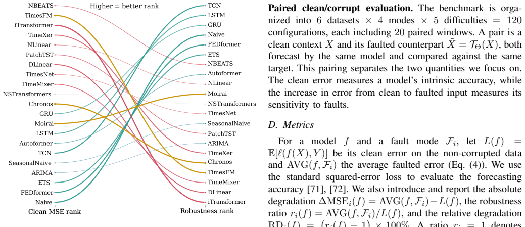
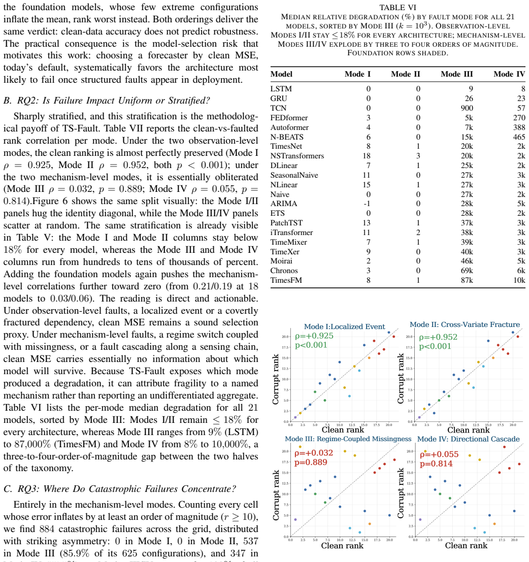
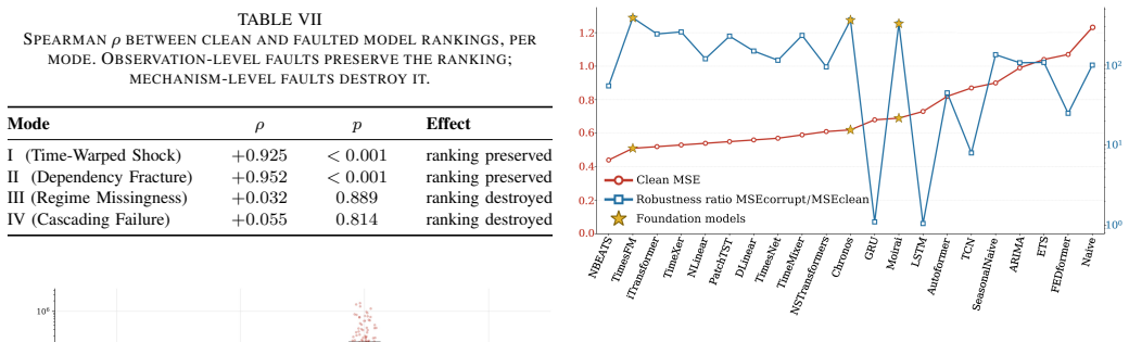
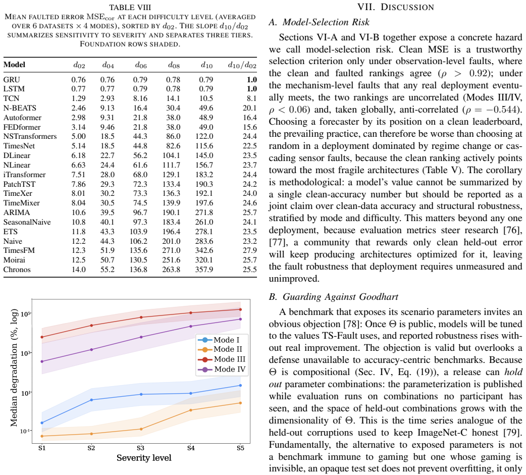
TS-Fault demonstrates that clean-data accuracy anti-correlates with robustness; clean rankings are preserved under observation-level faults but reshuffled under mechanism-level faults; and all catastrophic failures occur under mechanism-level faults, with foundation models achieving the highest clean-data accuracy yet exhibiting the greatest fragility.
What carries the argument
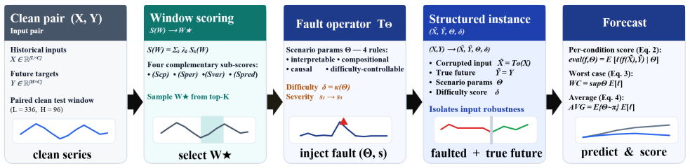
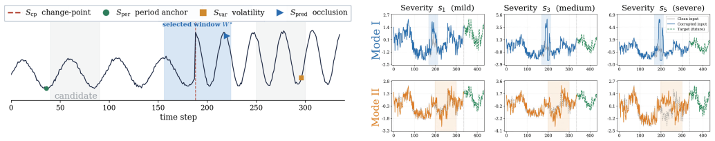
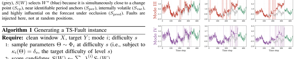
The TS-Fault benchmark that organizes recurring failures into four modes along observation-versus-mechanism and univariate-versus-multivariate axes and places each fault into the most prediction-critical window via a unified importance score.
If this is right
- Models must be tested under paired clean and faulted conditions rather than clean data alone.
- Observation-level faults leave existing clean rankings intact while mechanism-level faults reorder them.
- Foundation models require separate robustness evaluation because they show the largest drop from clean to faulted performance.
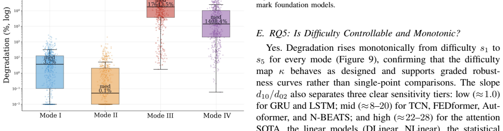
- Benchmarking should prioritize mechanism-level faults since they alone produce catastrophic failures.
Where Pith is reading between the lines
- Selection of deployed forecasters may need separate robustness criteria instead of relying on public leaderboards.
- The benchmark protocol could be applied to new fault types if they can be expressed in the same four-mode structure.
- Training procedures that improve clean accuracy may need explicit penalties for mechanism-level fragility.
Load-bearing premise
The four defined fault modes and the importance score for placing faults actually capture the structures that deployed forecasting models rely on rather than arbitrary synthetic corruptions.
What would settle it
A dataset or set of deployed logs in which the ranking of models by clean accuracy matches their ranking by robustness under the four fault modes, or real faults that produce model behavior outside the four modes.
Figures
read the original abstract
Time series forecasting (TSF) underpins consequential decisions in energy, transportation, finance, and healthcare, yet TSF models are almost universally ranked by a single number (e.g., average error) on clean held-out data, under the implicit assumption that it predicts deployed reliability. However, real faults are not i.i.d noise but structured events with temporal shape, broken cross-variable dependencies, regime change coupled with missingness, and causal propagation across a sensing pipeline. Treating TSF robustness as a data-quality problem, we present TS-Fault, a benchmark that evaluates forecasting models under explicit, parameterized fault scenarios with controllable semantic difficulty. TS-Fault organizes recurring failures into four modes along two orthogonal axes (observation- vs mechanism-level; univariate vs multivariate) and injects each fault into the most prediction-critical window via a unified importance score. This design enables robustness to be tested against the structures models actually rely on, rather than reduced to generic noise sensitivity. We evaluate 21 models across 6 datasets, 4 modes, and 5 difficulty levels under a paired clean/corrupt protocol. The results reveal three findings that contradict common leaderboard intuition: (i) clean-data accuracy anti-correlates with robustness; (ii) clean rankings are preserved under observation-level faults but reshuffled under mechanism-level faults; and (iii) all catastrophic failures occur under mechanism-level faults, with foundation models achieving the highest clean-data accuracy yet exhibiting the greatest fragility. The code is publicly available at https://github.com/Ray-zyy/TS-Fault.
Editorial analysis
A structured set of objections, weighed in public.
Referee Report
Summary. The paper introduces TS-Fault, a benchmark that organizes recurring TSF failures into four fault modes (observation- vs. mechanism-level crossed with univariate vs. multivariate) and injects each at high-importance windows via a unified importance score. It evaluates 21 models on 6 datasets across 4 modes and 5 difficulty levels under a paired clean/corrupt protocol, reporting that clean-data accuracy anti-correlates with robustness, that clean rankings are preserved under observation-level faults but reshuffled under mechanism-level faults, and that all catastrophic failures occur under mechanism-level faults (with foundation models most fragile).
Significance. If the four parameterized modes and importance-based placement are shown to be representative of real structural faults, the benchmark would provide concrete evidence against the assumption that clean-data leaderboards predict deployed reliability and would highlight mechanism-level faults as particularly diagnostic. Public code release is a clear strength for reproducibility.
major comments (2)
- [Abstract] Abstract: the assertion that the benchmark 'enables robustness to be tested against the structures models actually rely on' is load-bearing for interpreting the three headline findings, yet no validation is supplied that the chosen temporal shapes, dependency breaks, regime changes, or causal propagations match the distribution of observed faults in the six domains.
- [§4] §4 (Experiments) and the fault-mode definitions: no equation, algorithm, or pseudocode is given for computing the unified importance score used to place faults, nor for parameterizing semantic difficulty; without these, it is impossible to verify that placement is independent of the evaluated models or that the five difficulty levels are comparable across modes.
minor comments (2)
- A table enumerating the 21 models, their categories (e.g., statistical, deep, foundation), and the 6 datasets would improve readability of the experimental setup.
- The paired clean/corrupt protocol is described at a high level; explicit pseudocode or a small worked example of how a single fault injection affects a forecast would clarify the evaluation pipeline.
Simulated Author's Rebuttal
We thank the referee for the constructive feedback. We address the two major comments below, indicating planned revisions where appropriate. The benchmark is positioned as a controlled, parameterized testbed motivated by recurring failure patterns rather than a statistical replica of real fault distributions.
read point-by-point responses
-
Referee: [Abstract] Abstract: the assertion that the benchmark 'enables robustness to be tested against the structures models actually rely on' is load-bearing for interpreting the three headline findings, yet no validation is supplied that the chosen temporal shapes, dependency breaks, regime changes, or causal propagations match the distribution of observed faults in the six domains.
Authors: We acknowledge that the manuscript provides no direct empirical validation (e.g., via fault logs or domain studies) that the injected shapes exactly match the empirical distribution of faults in the six domains. The four modes are instead synthesized from documented recurring failure patterns reported in the TSF literature for energy, transportation, finance, and healthcare. We will revise the abstract and add a dedicated paragraph in §2 (Related Work) and §5 (Discussion) that (a) explicitly cites domain-specific studies on structural faults and (b) clarifies that the benchmark tests robustness against representative structures rather than claiming distributional equivalence. This addresses the load-bearing claim without requiring new data collection. revision: partial
-
Referee: [§4] §4 (Experiments) and the fault-mode definitions: no equation, algorithm, or pseudocode is given for computing the unified importance score used to place faults, nor for parameterizing semantic difficulty; without these, it is impossible to verify that placement is independent of the evaluated models or that the five difficulty levels are comparable across modes.
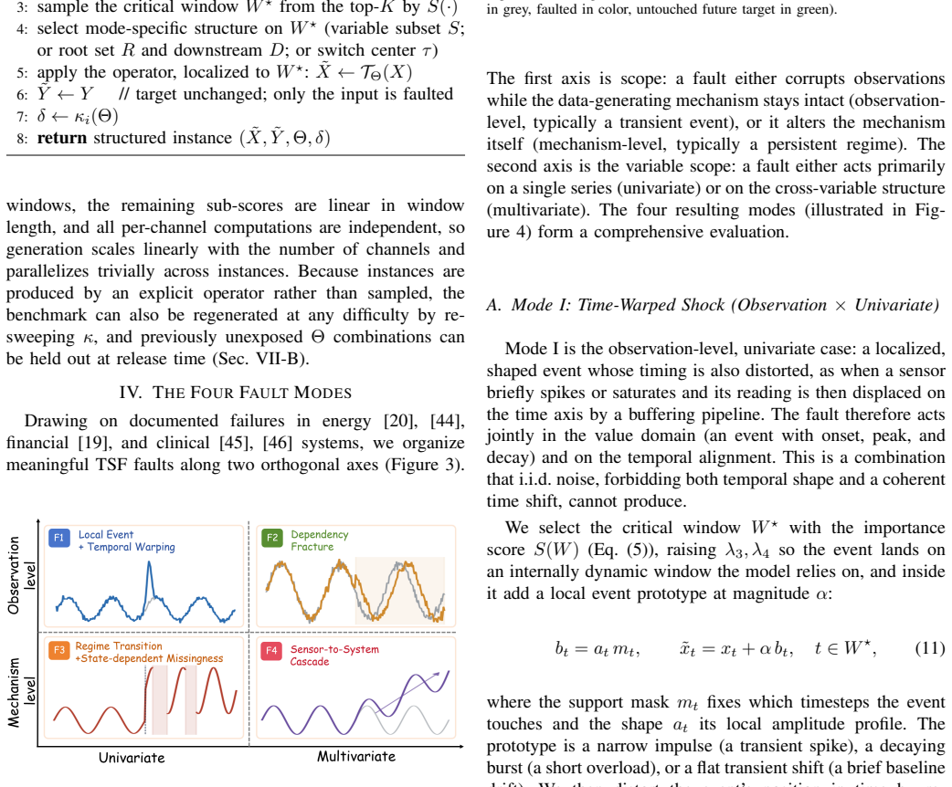
Authors: This observation is correct; the current manuscript describes the importance score at a high level but omits the formal definition, computation steps, and parameterization. In the revision we will insert (i) the exact equation for the unified importance score (a model-agnostic weighted combination of gradient saliency, temporal variance, and cross-variable dependency strength, averaged over a small held-out set of models), (ii) the algorithm for selecting the top-k windows, and (iii) the parameterization table that maps semantic difficulty levels to concrete fault parameters (e.g., missingness rate, regime-shift magnitude) for each mode. Pseudocode will be added to §4 to demonstrate that placement is independent of any single evaluated model and that difficulty levels are defined comparably across modes. revision: yes
Circularity Check
No significant circularity; empirical benchmark independent of findings
full rationale
The paper defines four synthetic fault modes (observation/mechanism, uni/multi) and an importance score for injection, then runs a paired clean/corrupt evaluation on 21 models across 6 datasets. The headline results (anti-correlation of clean accuracy with robustness, ranking preservation under observation faults, all catastrophes under mechanism faults) are direct empirical outputs of this protocol. No equations, fitted parameters, or self-citations reduce the robustness scores to quantities defined by the clean-data rankings or by construction. The benchmark construction stands as an independent experimental design rather than a self-referential derivation.
Axiom & Free-Parameter Ledger
free parameters (1)
- importance score parameters
axioms (1)
- domain assumption Real faults in deployed time series pipelines exhibit observation-level versus mechanism-level structure and univariate versus multivariate patterns.
Reference graph
Works this paper leans on
-
[1]
Modelardb: Modu- lar model-based time series management with spark and cassandra,
S. K. Jensen, T. B. Pedersen, and C. Thomsen, “Modelardb: Modu- lar model-based time series management with spark and cassandra,” PVLDB, vol. 11, no. 11, pp. 1688–1701, 2018
2018
-
[2]
Camel: Efficient compression of floating-point time series,
Y . Yao, L. Chen, Z. Fang, Y . Gao, C. S. Jensen, and T. Li, “Camel: Efficient compression of floating-point time series,”SIGMOD, vol. 2, no. 6, pp. 1–26, 2025
2025
-
[3]
Short-term traffic forecasting: Where we are and where we’re going,
E. I. Vlahogianni, M. G. Karlaftis, and J. C. Golias, “Short-term traffic forecasting: Where we are and where we’re going,”TRANSPORT RES C-EMER, vol. 43, no. 1, pp. 3–19, 2014
2014
-
[4]
Fedformer: Frequency enhanced decomposed transformer for long-term series fore- casting,
T. Zhou, Z. Ma, Q. Wen, X. Wang, L. Sun, and R. Jin, “Fedformer: Frequency enhanced decomposed transformer for long-term series fore- casting,” inICML, 2022, pp. 27 268–27 286
2022
-
[5]
Tfb: Towards comprehensive and fair benchmarking of time series forecasting methods,
X. Qiu, J. Hu, L. Zhou, X. Wu, J. Du, B. Zhang, C. Guo, A. Zhou, C. S. Jensen, Z. Sheng, and B. Yang, “Tfb: Towards comprehensive and fair benchmarking of time series forecasting methods,”PVLDB, vol. 17, no. 9, pp. 2363–2377, 2024
2024
-
[6]
Probabilistic electric load forecasting: A tutorial review,
T. Hong and S. Fan, “Probabilistic electric load forecasting: A tutorial review,”Int. J. Forecast., vol. 32, no. 3, pp. 914–938, 2016
2016
-
[7]
Recent advances in electricity price forecasting: A review of probabilistic forecasting,
J. Nowotarski and R. Weron, “Recent advances in electricity price forecasting: A review of probabilistic forecasting,”RSER, vol. 81, no. 1, pp. 1548–1568, 2018
2018
-
[8]
Deep ehr: a survey of recent advances in deep learning techniques for electronic health record (ehr) analysis,
B. Shickel, P. J. Tighe, A. Bihorac, and P. Rashidi, “Deep ehr: a survey of recent advances in deep learning techniques for electronic health record (ehr) analysis,”IEEE J-BHI, vol. 22, no. 5, pp. 1589–1604, 2017
2017
-
[9]
Time series prediction using deep learning methods in healthcare,
M. A. Morid, O. R. L. Sheng, and J. Dunbar, “Time series prediction using deep learning methods in healthcare,”TMIS, vol. 14, no. 1, pp. 1–29, 2023
2023
-
[10]
Financial time series forecasting with deep learning: A systematic literature review: 2005–2019,
O. B. Sezer, M. U. Gudelek, and A. M. Ozbayoglu, “Financial time series forecasting with deep learning: A systematic literature review: 2005–2019,”ASOC, vol. 90, p. 106181, 2020
2005
-
[11]
The m3-competition: results, conclusions and implications,
S. Makridakis and M. Hibon, “The m3-competition: results, conclusions and implications,”Int. J. Forecast., vol. 16, no. 4, pp. 451–476, 2000
2000
-
[12]
The m4 competi- tion: 100,000 time series and 61 forecasting methods,
S. Makridakis, E. Spiliotis, and V . Assimakopoulos, “The m4 competi- tion: 100,000 time series and 61 forecasting methods,”Int. J. Forecast., vol. 36, no. 1, pp. 54–74, 2020
2020
-
[13]
Monash time series forecasting archive,
R. W. Godahewa, C. Bergmeir, G. I. Webb, R. Hyndman, and P. Montero-Manso, “Monash time series forecasting archive,” in NeurIPS, 2021
2021
-
[14]
Gift-eval: A benchmark for general time series forecasting model evaluation,
T. Aksu, G. Woo, J. Liu, X. Liu, C. Liu, S. Savarese, C. Xiong, and D. Sahoo, “Gift-eval: A benchmark for general time series forecasting model evaluation,”NeurIPS Workshop, 2024
2024
-
[15]
Robusttsf: Towards theory and design of robust time series forecasting with anomalies,
H. Cheng, Q. Wen, Y . Liu, and L. Sun, “Robusttsf: Towards theory and design of robust time series forecasting with anomalies,” inICLR, 2024, pp. 5787–5813
2024
-
[16]
Saits: Self-attention-based imputation for time series,
W. Du, D. C ˆot´e, and Y . Liu, “Saits: Self-attention-based imputation for time series,”ESWA, vol. 219, p. 119619, 2023
2023
-
[17]
Explaining and harnessing adversarial examples,
I. J. Goodfellow, J. Shlens, and C. Szegedy, “Explaining and harnessing adversarial examples,”ICLR, 2015
2015
-
[18]
Towards deep learning models resistant to adversarial attacks,
A. Madry, A. Makelov, L. Schmidt, D. Tsipras, and A. Vladu, “Towards deep learning models resistant to adversarial attacks,”arXiv preprint arXiv:1706.06083, 2017
Pith/arXiv arXiv 2017
-
[19]
No contagion, only interdependence: measuring stock market comovements,
K. J. Forbes and R. Rigobon, “No contagion, only interdependence: measuring stock market comovements,”J Finance, vol. 57, no. 5, pp. 2223–2261, 2002
2002
-
[20]
Cascading risks: Understanding the 2021 winter blackout in texas,
J. W. Busby, K. Baker, M. D. Bazilian, A. Q. Gilbert, E. Grubert, V . Rai, J. D. Rhodes, S. Shidore, C. A. Smith, and M. E. Webber, “Cascading risks: Understanding the 2021 winter blackout in texas,”Energy Res. Social Sci., vol. 77, no. 1, p. 102106, 2021
2021
-
[21]
Informer: Beyond efficient transformer for long sequence time-series forecasting,
H. Zhou, S. Zhang, J. Peng, S. Zhang, J. Li, H. Xiong, and W. Zhang, “Informer: Beyond efficient transformer for long sequence time-series forecasting,” inAAAI, vol. 35, no. 12, 2021, pp. 11 106–11 115
2021
-
[22]
Exploring progress in multivariate time series forecasting: Comprehensive benchmarking and heterogeneity analysis,
Z. Shao, F. Wang, Y . Xu, W. Wei, C. Yu, Z. Zhang, D. Yao, T. Sun, G. Jin, X. Caoet al., “Exploring progress in multivariate time series forecasting: Comprehensive benchmarking and heterogeneity analysis,” TKDE, vol. 37, no. 1, pp. 291–305, 2024
2024
-
[23]
fev-bench: A realistic benchmark for time series forecasting,
O. Shchur, A. F. Ansari, C. Turkmen, L. Stella, N. Erickson, P. Guerron, M. Bohlke-Schneider, and Y . Wang, “fev-bench: A realistic benchmark for time series forecasting,”arXiv preprint arXiv:2509.26468, 2025
arXiv 2025
-
[24]
Tsfm-bench: A comprehensive and unified benchmark of foundation models for time series forecasting,
Z. Li, X. Qiu, P. Chen, Y . Wang, H. Cheng, Y . Shu, J. Hu, C. Guo, A. Zhou, C. S. Jensenet al., “Tsfm-bench: A comprehensive and unified benchmark of foundation models for time series forecasting,” inSIGKDD, 2025, pp. 5595–5606
2025
-
[25]
Probts: Benchmarking point and distributional forecasting across diverse pre- diction horizons,
J. Zhang, X. Wen, Z. Zhang, S. Zheng, J. Li, and J. Bian, “Probts: Benchmarking point and distributional forecasting across diverse pre- diction horizons,” inNeurIPS, vol. 37, 2024, pp. 48 045–48 082
2024
-
[26]
Scaling laws for neural language models,
J. Kaplan, S. McCandlish, T. Henighan, T. B. Brown, B. Chess, R. Child, S. Gray, A. Radford, J. Wu, and D. Amodei, “Scaling laws for neural language models,”arXiv preprint arXiv:2001.08361, 2020
Pith/arXiv arXiv 2001
-
[27]
Training compute-optimal large language models,
J. Hoffmann, S. Borgeaud, A. Mensch, E. Buchatskaya, T. Cai, E. Rutherford, D. Casas, L. A. Hendricks, J. Welbl, A. Clarket al., “Training compute-optimal large language models,”NeurIPS, 2022
2022
-
[28]
Chronos: Learning the language of time series,
A. F. Ansari, L. Stella, C. Turkmen, X. Zhang, P. Mercado, H. Shen, O. Shchur, S. S. Rangapuram, S. P. Arango, S. Kapooret al., “Chronos: Learning the language of time series,”TMLR, 2024
2024
-
[29]
A decoder-only foundation model for time-series forecasting,
A. Das, W. Kong, R. Sen, and Y . Zhou, “A decoder-only foundation model for time-series forecasting,”ICML, 2024
2024
-
[30]
Unified training of universal time series forecasting transformers,
G. Woo, C. Liu, A. Kumar, C. Xiong, S. Savarese, and D. Sahoo, “Unified training of universal time series forecasting transformers,” in ICML, 2024
2024
-
[31]
Foundation models for time series analysis: A tutorial and survey,
Y . Liang, H. Wen, Y . Nie, Y . Jiang, M. Jin, D. Song, S. Pan, and Q. Wen, “Foundation models for time series analysis: A tutorial and survey,” in SIGKDD, 2024, pp. 6555–6565
2024
-
[32]
Nlp evaluation in trouble: On the need to measure llm data contamination for each benchmark,
O. Sainz, J. Campos, I. Garc ´ıa-Ferrero, J. Etxaniz, O. L. de Lacalle, and E. Agirre, “Nlp evaluation in trouble: On the need to measure llm data contamination for each benchmark,” inEMNLP Findings, 2023, pp. 10 776–10 787
2023
-
[33]
Time travel in llms: Tracing data contamination in large language models,
S. Golchin and M. Surdeanu, “Time travel in llms: Tracing data contamination in large language models,”ICLR, 2024
2024
-
[34]
Benchmark data contamination of large language models: A survey,
C. Xu, S. Guan, D. Greene, M. Kechadiet al., “Benchmark data contamination of large language models: A survey,”arXiv preprint arXiv:2406.04244, 2024
Pith/arXiv arXiv 2024
-
[35]
Brits: Bidirectional recurrent imputation for time series,
W. Cao, D. Wang, J. Li, H. Zhou, L. Li, and Y . Li, “Brits: Bidirectional recurrent imputation for time series,”NeurIPS, vol. 31, pp. 6776–6786, 2018
2018
-
[36]
Wild-time: A benchmark of in-the-wild distribution shift over time,
H. Yao, C. Choi, B. Cao, Y . Lee, P. W. W. Koh, and C. Finn, “Wild-time: A benchmark of in-the-wild distribution shift over time,” inNeurIPS, vol. 35, 2022, pp. 10 309–10 324
2022
-
[37]
Woods: Benchmarks for out-of-distribution generalization in time series,
J.-C. Gagnon-Audet, K. Ahuja, M.-J. Darvishi-Bayazi, P. Mousavi, G. Dumas, and I. Rish, “Woods: Benchmarks for out-of-distribution generalization in time series,”TMLR, 2023
2023
-
[38]
Wilds: A benchmark of in-the-wild distribution shifts,
P. W. Koh, S. Sagawa, H. Marklund, S. M. Xie, M. Zhang, A. Balsub- ramani, W. Hu, M. Yasunaga, R. L. Phillips, I. Gaoet al., “Wilds: A benchmark of in-the-wild distribution shifts,” inICML, 2021, pp. 5637– 5664
2021
-
[39]
Benchmarking neural network robust- ness to common corruptions and perturbations,
D. Hendrycks and T. Dietterich, “Benchmarking neural network robust- ness to common corruptions and perturbations,”ICLR, 2019
2019
-
[40]
Toward causal representation learning,
B. Sch ¨olkopf, F. Locatello, S. Bauer, N. R. Ke, N. Kalchbrenner, A. Goyal, and Y . Bengio, “Toward causal representation learning,”Proc. IEEE, vol. 109, no. 5, pp. 612–634, 2021
2021
-
[41]
Peters, D
J. Peters, D. Janzing, and B. Scholkopf,Elements of causal inference: foundations and learning algorithms. MIT press, 2017
2017
-
[42]
A survey of methods for time series change point detection,
S. Aminikhanghahi and D. J. Cook, “A survey of methods for time series change point detection,”KAIS, vol. 51, no. 2, pp. 339–367, 2017
2017
-
[43]
Hot sax: Efficiently finding the most unusual time series subsequence,
E. Keogh, J. Lin, and A. Fu, “Hot sax: Efficiently finding the most unusual time series subsequence,” inICDM, 2005, pp. 8–pp
2005
-
[44]
Causes of the 2003 major grid blackouts in north america and europe, and recommended means to improve system dynamic performance,
G. Andersson, P. Donalek, R. Farmer, N. Hatziargyriou, I. Kamwa, P. Kundur, N. Martins, J. Paserba, P. Pourbeik, J. Sanchez-Gascaet al., “Causes of the 2003 major grid blackouts in north america and europe, and recommended means to improve system dynamic performance,”T- PWRS, vol. 20, no. 4, pp. 1922–1928, 2005
2003
-
[45]
Early prediction of sepsis in the icu using machine learning: a systematic review,
M. Moor, B. Rieck, M. Horn, C. R. Jutzeler, and K. Borgwardt, “Early prediction of sepsis in the icu using machine learning: a systematic review,”Front. Med., vol. 8, p. 607952, 2021
2021
-
[46]
Time to treatment and mortality during mandated emergency care for sepsis,
C. W. Seymour, F. Gesten, H. C. Prescott, M. E. Friedrich, T. J. Iwashyna, G. S. Phillips, S. Lemeshow, T. Osborn, K. M. Terry, and M. M. Levy, “Time to treatment and mortality during mandated emergency care for sepsis,”NEJM, vol. 376, no. 23, pp. 2235–2244, 2017
2017
-
[47]
R. J. Little and D. B. Rubin,Statistical analysis with missing data. John Wiley & Sons, 2019
2019
-
[48]
A cross-domain approach to analyzing the short-run impact of covid-19 on the us electricity sector,
G. Ruan, D. Wu, X. Zheng, H. Zhong, C. Kang, M. A. Dahleh, S. Sivaranjani, and L. Xie, “A cross-domain approach to analyzing the short-run impact of covid-19 on the us electricity sector,”Joule, vol. 4, no. 11, pp. 2322–2337, 2020
2020
-
[49]
Complex systems analysis of series of blackouts: Cascading failure, critical points, and self-organization,
I. Dobson, B. A. Carreras, V . E. Lynch, and D. E. Newman, “Complex systems analysis of series of blackouts: Cascading failure, critical points, and self-organization,”Chaos, vol. 17, no. 2, 2007
2007
-
[50]
Catastrophic cascade of failures in interdependent networks,
S. V . Buldyrev, R. Parshani, G. Paul, H. E. Stanley, and S. Havlin, “Catastrophic cascade of failures in interdependent networks,”Nature, vol. 464, no. 7291, pp. 1025–1028, 2010
2010
-
[51]
Reliability standards for the bulk electric systems of north america,
N. A. E. R. Corporation, “Reliability standards for the bulk electric systems of north america,” 2018
2018
-
[52]
Analysis of the blackout in europe on november 4, 2006,
C. Li, Y . Sun, and X. Chen, “Analysis of the blackout in europe on november 4, 2006,”IPEC, pp. 939–944, 2007
2006
-
[53]
Autoformer: Decomposition transformers with auto-correlation for long-term series forecasting,
H. Wu, J. Xu, J. Wang, and M. Long, “Autoformer: Decomposition transformers with auto-correlation for long-term series forecasting,” in NeurIPS, vol. 34, 2021, pp. 22 419–22 430
2021
-
[54]
Modeling long-and short- term temporal patterns with deep neural networks,
G. Lai, W.-C. Chang, Y . Yang, and H. Liu, “Modeling long-and short- term temporal patterns with deep neural networks,” inSIGIR, 2018, pp. 95–104
2018
-
[55]
TSMixer: An all-MLP architecture for time series forecast-ing,
S.-A. Chen, C.-L. Li, S. O. Arik, N. C. Yoder, and T. Pfister, “TSMixer: An all-MLP architecture for time series forecast-ing,”TMLR, 2023
2023
-
[56]
A time series is worth 64 words: Long-term forecasting with transformers,
Y . Nie, N. H. Nguyen, P. Sinthong, and J. Kalagnanam, “A time series is worth 64 words: Long-term forecasting with transformers,” inICLR, 2023
2023
-
[57]
Multi-resolution time-series transformer for long-term forecasting,
Y . Zhang, L. Ma, S. Pal, Y . Zhang, and M. Coates, “Multi-resolution time-series transformer for long-term forecasting,” inAISTATS, vol. 238, 2024, pp. 4222–4230
2024
-
[58]
R. J. Hyndman and G. Athanasopoulos,Forecasting: principles and practice. OTexts, 2018
2018
-
[59]
G. E. Box, G. M. Jenkins, G. C. Reinsel, and G. M. Ljung,Time series analysis: forecasting and control. John Wiley & Sons, 2015
2015
-
[60]
Hyndman, A
R. Hyndman, A. Koehler, K. Ord, and R. Snyder,Forecasting with exponential smoothing: the state space approach. Springer, 2008
2008
-
[61]
Are transformers effective for time series forecasting?
A. Zeng, M. Chen, L. Zhang, and Q. Xu, “Are transformers effective for time series forecasting?” inAAAI, vol. 37, no. 9, 2023, pp. 11 121– 11 128
2023
-
[62]
N-beats: Neural basis expansion analysis for interpretable time series forecasting,
B. N. Oreshkin, D. Carpov, N. Chapados, and Y . Bengio, “N-beats: Neural basis expansion analysis for interpretable time series forecasting,” inICLR, 2020
2020
-
[63]
Long short-term memory,
S. Hochreiter and J. Schmidhuber, “Long short-term memory,”Neural Comput., vol. 9, no. 8, pp. 1735–1780, 1997
1997
-
[64]
Learning phrase representations using rnn encoder–decoder for statistical machine translation,
K. Cho, B. Van Merri ¨enboer, C ¸ . Gulc ¸ehre, D. Bahdanau, F. Bougares, H. Schwenk, and Y . Bengio, “Learning phrase representations using rnn encoder–decoder for statistical machine translation,” inEMNLP, 2014, pp. 1724–1734
2014
-
[65]
An empirical evaluation of generic convolutional and recurrent networks for sequence modeling,
S. Bai, J. Z. Kolter, and V . Koltun, “An empirical evaluation of generic convolutional and recurrent networks for sequence modeling,”arXiv preprint arXiv:1803.01271, 2018
Pith/arXiv arXiv 2018
-
[66]
itrans- former: Inverted transformers are effective for time series forecasting,
Y . Liu, T. Hu, H. Zhang, H. Wu, S. Wang, L. Ma, and M. Long, “itrans- former: Inverted transformers are effective for time series forecasting,” inICLR, vol. 2024, 2024, pp. 11 116–11 140
2024
-
[67]
Timexer: Empowering transformers for time series forecast- ing with exogenous variables,
Y . Wang, H. Wu, J. Dong, Y . Liu, Y . Qiu, H. Zhang, J. Wang, and M. Long, “Timexer: Empowering transformers for time series forecast- ing with exogenous variables,” inNeurIPS, vol. 37, 2024, pp. 469–498
2024
-
[68]
Timemixer: Decomposable multiscale mixing for time series forecasting,
S. Wang, H. Wu, X. Shi, T. Hu, H. Luo, L. Ma, J. Zhang, and J. Zhou, “Timemixer: Decomposable multiscale mixing for time series forecasting,” inICLR, vol. 2024, 2024, pp. 38 626–38 652
2024
-
[69]
Timesnet: Temporal 2d-variation modeling for general time series analysis,
H. Wu, T. Hu, Y . Liu, H. Zhou, J. Wang, and M. Long, “Timesnet: Temporal 2d-variation modeling for general time series analysis,” in ICLR, 2023
2023
-
[70]
Non-stationary transformers: Exploring the stationarity in time series forecasting,
Y . Liu, H. Wu, J. Wang, and M. Long, “Non-stationary transformers: Exploring the stationarity in time series forecasting,” inNeurIPS, vol. 35, 2022, pp. 9881–9893
2022
-
[71]
Another look at measures of forecast accuracy,
R. J. Hyndman and A. B. Koehler, “Another look at measures of forecast accuracy,”Int. J. Forecast., vol. 22, no. 4, pp. 679–688, 2006
2006
-
[72]
Strictly proper scoring rules, prediction, and estimation,
T. Gneiting and A. E. Raftery, “Strictly proper scoring rules, prediction, and estimation,”J Am Stat Assoc., vol. 102, no. 477, pp. 359–378, 2007
2007
-
[73]
Shortcut learning in deep neural networks,
R. Geirhos, J.-H. Jacobsen, C. Michaelis, R. Zemel, W. Brendel, M. Bethge, and F. A. Wichmann, “Shortcut learning in deep neural networks,”Nat. Mach. Intell., vol. 2, no. 11, pp. 665–673, 2020
2020
-
[74]
Underspec- ification presents challenges for credibility in modern machine learning,
A. D’Amour, K. Heller, D. Moldovan, B. Adlam, B. Alipanahi, A. Beu- tel, C. Chen, J. Deaton, J. Eisenstein, M. D. Hoffmanet al., “Underspec- ification presents challenges for credibility in modern machine learning,” JMLR, vol. 23, no. 226, pp. 1–61, 2022
2022
-
[75]
Reversible instance normalization for accurate time-series forecasting against dis- tribution shift,
T. Kim, J. Kim, Y . Tae, C. Park, J.-H. Choi, and J. Choo, “Reversible instance normalization for accurate time-series forecasting against dis- tribution shift,” inICLR, 2021
2021
-
[76]
Beyond accuracy: Behavioral testing of nlp models with checklist,
M. T. Ribeiro, T. Wu, C. Guestrin, and S. Singh, “Beyond accuracy: Behavioral testing of nlp models with checklist,” inACL, 2020, pp. 4902–4912
2020
-
[77]
Dynabench: Rethinking benchmarking in nlp,
D. Kiela, M. Bartolo, Y . Nie, D. Kaushik, A. Geiger, Z. Wu, B. Vid- gen, G. Prasad, A. Singh, P. Ringshiaet al., “Dynabench: Rethinking benchmarking in nlp,” inNAACL, 2021, pp. 4110–4124
2021
-
[78]
Categorizing variants of goodhart’s law,
D. Manheim and S. Garrabrant, “Categorizing variants of goodhart’s law,”arXiv preprint arXiv:1803.04585, 2018
Pith/arXiv arXiv 2018
-
[79]
On interaction between augmen- tations and corruptions in natural corruption robustness,
E. Mintun, A. Kirillov, and S. Xie, “On interaction between augmen- tations and corruptions in natural corruption robustness,” inNeurIPS, vol. 34, 2021, pp. 3571–3583
2021
-
[80]
Anomaly detection: A survey,
V . Chandola, A. Banerjee, and V . Kumar, “Anomaly detection: A survey,” CSUR, vol. 41, no. 3, pp. 1–58, 2009
2009
discussion (0)
Sign in with ORCID, Apple, or X to comment. Anyone can read and Pith papers without signing in.