REVIEW 4 major objections 6 minor 32 references
DEF: Diffusion-augmented Ensemble Forecasting
T0 review · 4 major / 6 minor · reviewed 2026-08-07 · deepseek-v4-flash
Pith's one-line read A small conditional diffusion model can perturb the initial conditions of any deterministic machine-learned weather forecaster, producing an ensemble whose mean beats the deterministic forecast and whose spread tracks error.
desk verdict A modular and genuinely new recipe for diffusion-based initial condition perturbations, but the reported gains are largely a predictor-corrector effect on a weak baseline—the model-agnostic claim is unproven. read the letter →
The pith
A machine-rendered reading of the paper's core claim, the machinery that carries it, and where it could break.
The reading
What carries the argument
The load-bearing object is the conditional denoising diffusion model $\epsilon_\theta(\tilde{x}_t, t, x_t)$ trained with the standard denoising objective and classifier-free guidance: at inference, guidance interpolates conditional and unconditional noise estimates as $\hat{\epsilon} = \epsilon_\theta(\tilde{x}_t,t,\emptyset)+\omega(\epsilon_\theta(\tilde{x}_t,t,x_t)-\epsilon_\theta(\tilde{x}_t,t,\emptyset))$. The same network, run through a fast DPM-Solver++ sampler, produces the initial-condition perturbations, while a separate deterministic forecaster $G_\phi$ advances each perturbed state; this decoupling is what lets the method wrap any deterministic predictor unchanged. Iterative application of the perturbation step creates the 'random walk' that increases exploration.
What would settle it
Run the same diffusion-perturbation pipeline on several start dates spread across seasons and years, holding the trained models fixed, and compare the ensemble-mean RMSE and spread to the deterministic baseline on each case; if the improvement over the deterministic run does not persist out-of-sample, or if the spread no longer tracks the error, the central claim fails. A simpler check is to verify in the ERA5 split used here whether January 12 of the chosen year falls inside the training window.
Extended reading notes
Core claim
The paper's central claim is that a classifier-free guided conditional diffusion model, operating directly on the current atmospheric state, is a sufficient and transferable perturbation mechanism for ensemble weather forecasting. Given an observed state, the diffusion model draws a small structured perturbation; the deterministic forecaster advances each perturbed state; repeating this process yields an ensemble. The paper further claims that the guidance scale $\omega$ gives intuitive control over perturbation strength, that iterating the perturbation before advancement ('random walks') explores the trajectory space, and that the diffusion step acts as a predictor-corrector, projecting model states back onto the learned data manifold and thereby suppressing out-of-domain values such as negative specific humidity. On the $5.625^\circ$ ERA5 subset, the ensemble mean beats the deterministic baseline on RMSE for the variables examined, most clearly for 2-meter temperature and specific humidity, while Energy Score, CRPS, and spread values indicate a usable forecast distribution.
Load-bearing premise
The quantitative case rests on a single 10-day forecast initialized on January 12, with no stated temporal separation between the training data and that window; if that start date falls inside the training period or is an atypically correctable case, the reported error reductions and spread values would not support the general claim.
Editorial extensions
If this is right
- Any deterministic ML weather predictor can be converted to a stochastic ensemble system by adding this perturbation module, without changing the predictor's architecture or training objective.
- The guidance parameter $\omega$ gives a user a single, interpretable dial for trading ensemble diversity against fidelity.
- Iterative perturbation steps increase exploration, equivalent to a random walk in state space, at the cost of larger spread and slightly higher RMSE.
- Because the diffusion step re-projects states onto the learned data distribution, ensemble members respect physical bounds and conserve domain-averaged energy better than the bare deterministic model.
- Probabilistic scores (Energy Score, CRPS) and spread are reported together with ensemble-mean skill, so the method can be assessed on calibration rather than point error alone.
Reading between the lines
- The method could be read as a stochastic regularizer: the diffusion projection removes unstable or out-of-domain states, so part of the accuracy gain may come from correction rather than from ensemble averaging; testing the projection with a single member would separate the two effects.
- If the approach transfers to strong predictors, the natural next comparison is against native stochastic models on standardized benchmarks, but the paper does not supply that evidence.
- The 'random walk' formulation suggests a connection to stochastic differential equation sampling of the forecast trajectory itself, which could be made rigorous by studying the limit of many small perturbation steps.
Editorial analysis
A structured set of objections, weighed in public.
Referee Report
Summary. The paper proposes DEF (Diffusion-augmented Ensemble Forecasting), a modular wrapper that aims to turn any deterministic autoregressive weather forecaster into a stochastic ensemble forecaster. At inference, a conditional denoising diffusion model is used to resample the current forecast state, the deterministic model advances that perturbed state, and the process is repeated; a classifier-free guidance weight controls perturbation strength and an iterative random-walk parameter K is explored. The method is evaluated on 5.625° ERA5 with a custom attention U-Net as the deterministic baseline, using one 240-hour forecast initialized on January 12 (year not stated). The authors report that the ensemble mean substantially reduces RMSE relative to the deterministic baseline, e.g., 2m temperature RMSE at 234h lead falls from 8.12 to 4.03, and they claim the approach can make any deterministic ML weather predictor stochastic. Code is publicly available under an open-source license.
Significance. If validated, DEF would be a genuinely useful modular contribution: it does not require retraining the deterministic forecaster, it is parallelizable, and the guidance term offers an intuitive control of perturbation strength. The paper has real strengths: an open-source repository, clear algorithmic appendices, an honest Limitations section, and a framing that addresses a genuine gap in MLWP ensemble generation. However, the evidence as submitted does not establish the central claim. The quantitative evaluation is a single 10-day case with no train/test temporal split and no error bars; the only baseline is the authors' own weak deterministic model that produces out-of-domain values; and the diffusion model is trained on a mixture of true states and G_theta outputs, so the reported gains are confounded with a predictor-corrector effect that the paper itself acknowledges. In addition, Eq. (20) and Algorithm 2 show that the diffusion model is applied at every lead time, not only to the initial condition, so the 'initial condition perturbation' framing is inaccurate.
major comments (4)
- [§4.2, Eq. (20) and Algorithm 2] The method is not an initial-condition perturbation as claimed in the title, abstract, and contribution (1). Equation (20) defines x_{t+1}^{(b)} = G_phi(tilde x_t^{(b)}) with tilde x_t^{(b)} = epsilon_theta(x_t^{(b)}), and Algorithm 2 applies the diffusion sampler to every state along the trajectory before each autoregressive step. This is a stochastic per-step state perturbation and manifold projection scheme, not an ensemble generated by perturbing only x_0. To support the stated contribution, the authors should either re-frame the method as stochastic state-space resampling or add an experimental variant where only the initial condition is perturbed and the trajectory is integrated deterministically thereafter.
- [§6, Algorithm 3, Table 3] The headline RMSE improvements are confounded with a predictor-corrector effect. Algorithm 3 lines 4-6 train epsilon_theta on a 50% mixture of true ERA5 states and states produced by G_theta, and Section 6 explicitly states that the method 'also acts as a predictor-corrector, projecting predictions onto a manifold learned from the data distribution.' Since Section 5 documents that the deterministic baseline produces negative specific humidity and out-of-bounds 2m temperatures, the large reductions in Table 3 (e.g., 8.12 to 4.03 at 234h for 2m temperature) may be due to repairing an invalid baseline rather than to the value of ensemble initial-condition diversity. The paper needs a correction-only control, e.g., applying epsilon_theta at every step with identical members and no stochasticity, and a well-behaved deterministic baseline such as GraphCast or FuXi, to separate the two effects.
- [§5 and §4.1] The entire quantitative evaluation rests on one start date. Section 5 states 'We do evaluation with the same start time of January 12th, 12 AM until January 22th, 12 AM,' and Section 4.1 gives no train/validation/test temporal split for ERA5. No error bars, no alternative initializations, and no significance tests are reported, so all headline numbers could reflect a single atypical or training-overlapping case. The authors should provide multi-initialization results over a defined test period (e.g., a seasonal or multi-year protocol) and report uncertainty estimates, which is load-bearing for the generalizable claim in the abstract.
- [§4.3, Eqs. (22)-(25), Tables 3 and B.4-B.14] The probabilistic claims are not supported by proper calibration evidence. Equation (25) defines 'Spread Correlation' as a norm of the difference between the forecast error and the ensemble standard deviation, which is not a correlation, and this quantity is never reported in Tables 3, B.4, or B.5-B.14. Reporting spread values alone does not establish a spread-skill relationship. The authors should provide proper calibration diagnostics, such as rank histograms, spread-error correlation as a function of lead time, and CRPS relative to a climatological or reference ensemble, and should correct the name and definition of the SC metric.
minor comments (6)
- [§4.2 and Algorithm 2] Equation (20) writes tilde x_t^{(b)} = epsilon_theta(x_t^{(b)}), but Algorithm 2 conditions the denoiser on x_{t-1} (line 10) and then sets tilde x_t <- z_0; the conditioning input in Eq. (20) is inconsistent with the algorithm and should be aligned.
- [Table 3 and Appendix B] The notation Diffusion[0.5, 1] is never defined; from the Appendix B tables it appears to denote [guidance scale w, number of iterative walks K], but this should be stated in the caption or at first use in Section 5.
- [§5, Figure 5] The text says Figure 5 demonstrates 'conservation of energy,' but the plotted domain-averaged values of 2m temperature or specific humidity are not energy quantities; the figure should be described as showing domain-averaged state values, not energy conservation.
- [Abstract and text] There are several typos and minor wording issues: 'intuitivey' in the Abstract, 'acheieve' in §3.4, 'January 22th' in §5, and '12 AM' should be replaced with an unambiguous UTC time. These should be corrected.
- [§3.2, Eqs. (3)-(4)] The perturbation function F is introduced in Eq. (4) but never used or connected to the diffusion model; the authors should either remove this formalism or explicitly relate F to epsilon_theta.
- [§6] The statement that RMSE is 'up to 50% lower on the high end and approximately 10% lower on the low end, after standardizing' is not directly supported by the tables, which report unstandardized RMSEs; the variables and standardization procedure used for this claim should be specified.
Circularity Check
Headline RMSE gains reduce to the diffusion model's trained predictor-corrector effect on the same Gθ baseline, so the central quantitative claim is partially circular.
-
fitted input called prediction
[Algorithm 3, lines 4-6; Section 6 Discussion; Limitations]
"s∼Bernoulli(0.5); if s=1 then x0 ← Gθ(x0){Advance sample through time} ... an additional benefit of using a diffusion model as a perturbation method is that it also acts as a predictor-corrector, projecting predictions onto a manifold learned from the data distribution."
Algorithm 3 trains the diffusion model with s∼Bernoulli(0.5) and, when s=1, replaces the target with Gθ(x0). The same Gθ is the deterministic baseline used at inference (Eq. 20). Consequently, the perturbation model has been fitted to map Gθ outputs back toward the ERA5 manifold, which the paper itself calls a 'predictor-corrector, projecting predictions onto a manifold learned from the data distribution.' The reported long-lead RMSE reductions (e.g., 8.12→4.03 in Table 3) are therefore largely the fitted correction of that specific weak baseline, not an independent IC-perturbation effect. No other deterministic predictor is tested, and the Limitations state the generalizability claim 'has not been empirically validated.'
full rationale
The paper's core methodological contribution—training a conditional diffusion model to generate state perturbations—is not itself circular. The circular concern is confined to the evaluation of the claim that this improves deterministic forecasts. Algorithm 3 explicitly trains the perturbation model on a 50/50 mix of true ERA5 states and states produced by the same deterministic model Gθ used in the experiments. During inference (Algorithm 2), the diffusion model is applied to the autoregressive Gθ trajectory at every step. The paper's own Section 6 states the method 'also acts as a predictor-corrector, projecting predictions onto a manifold learned from the data distribution.' Thus the RMSE reductions in Table 3 (e.g., 2m temperature from 8.12 to 4.03 at 234h) are substantially a fitted correction of the weak, out-of-domain baseline, as the paper acknowledges (negative specific humidity, implausible temperatures). This does not by itself invalidate the perturbation idea, but it means the reported quantitative claim is partly 'prediction' of what was trained in. The model-agnostic generalization claim ('transforming any deterministic neural forecasting system') is explicitly flagged in the Limitations as not empirically validated, and only one start date (Jan 12) is evaluated with no explicit temporal split. These are correctness/scope risks rather than additional circular steps. Overall, one load-bearing evaluation step reduces by construction to the training setup, so the score is 6 rather than a clean non-finding.
Assumptions & free parameters
free parameters (5)
- guidance scale w =
0.3, 0.5, 0.7, 1.0 (best often 0.5; 0.7 for geopotential)
- number of iterative walks K =
1, 3, 7
- diffusion sampling steps S (DPM++ solver) =
not stated
- classifier-free guidance dropout probability lambda =
not stated
- gradient clipping threshold tau =
not stated
assumptions (5)
- domain assumption ERA5 reanalysis states are treated as ground truth.
- domain assumption Samples from the conditional diffusion model represent plausible initial states consistent with forecast uncertainty.
- ad hoc to paper Training on a mix of true states and G_theta outputs makes the diffusion model a sufficient corrector for the same model at long lead times.
- ad hoc to paper The single January 12-22 evaluation window is representative and out-of-sample.
- standard math Standard DDPM, classifier-free guidance, and DPM-Solver results are correct.
Cite this review
Pith. "Pith review of DEF: Diffusion-augmented Ensemble Forecasting." pith.science (2026). https://pith.science/paper/H7JNVJSQ
@misc{pith2026250607324,
  author       = {Pith},
  title        = {Pith review of: DEF: Diffusion-augmented Ensemble Forecasting},
  year         = {2026},
  howpublished = {\url{https://pith.science/paper/H7JNVJSQ}},
  note         = {Machine review of arXiv:2506.07324}
}
abstract
We present DEF (\textbf{\ul{D}}iffusion-augmented \textbf{\ul{E}}nsemble \textbf{\ul{F}}orecasting), a novel approach for generating initial condition perturbations. Modern approaches to initial condition perturbations are primarily designed for numerical weather prediction (NWP) solvers, limiting their applicability in the rapidly growing field of machine learning for weather prediction. Consequently, stochastic models in this domain are often developed on a case-by-case basis. We demonstrate that a simple conditional diffusion model can (1) generate meaningful structured perturbations, (2) be applied iteratively, and (3) utilize a guidance term to intuitivey control the level of perturbation. This method enables the transformation of any deterministic neural forecasting system into a stochastic one. With our stochastic extended systems, we show that the model accumulates less error over long-term forecasts while producing meaningful forecast distributions. We validate our approach on the 5.625$^\circ$ ERA5 reanalysis dataset, which comprises atmospheric and surface variables over a discretized global grid, spanning from the 1960s to the present. On this dataset, our method demonstrates improved predictive performance along with reasonable spread estimates.
Figures


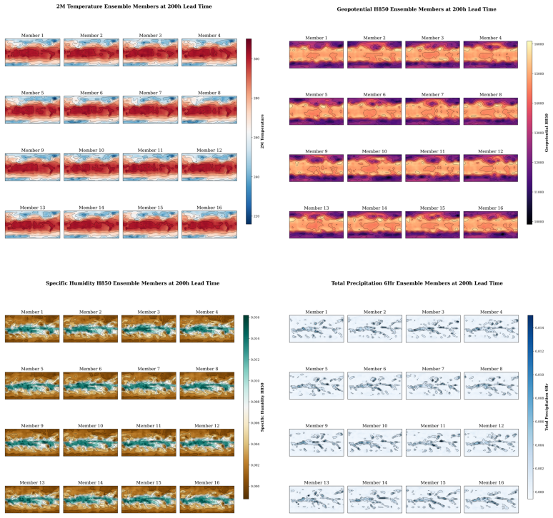
Figures from the paper (2 more)

Reference graph
Works this paper leans on
-
[1]
K. Bi, L. Xie, H. Zhang, X. Chen, X. Gu, Q. Tian, Pangu-weather: A 3d high- resolution model for fast and accurate global weather forecast (2022).arXiv:2211. 02556. URLhttps://arxiv.org/abs/2211.02556
arXiv 2022
-
[2]
R. Lam, A. Sanchez-Gonzalez, M. Willson, P. Wirnsberger, M. Fortunato, F. Alet, S. Ravuri, T. Ewalds, Z. Eaton-Rosen, W. Hu, A. Merose, S. Hoyer, G. Holland, O. Vinyals, J. Stott, A. Pritzel, S. Mohamed, P. Battaglia, Graphcast: Learning skillful medium-range global weather forecasting (2023).arXiv:2212.12794. URLhttps://arxiv.org/abs/2212.12794
arXiv 2023
-
[3]
J. Pathak, S. Subramanian, P. Harrington, S. Raja, A. Chattopadhyay, M. Mar- dani, T. Kurth, D. Hall, Z. Li, K. Azizzadenesheli, P. Hassanzadeh, K. Kashinath, A. Anandkumar, Fourcastnet: A global data-driven high-resolution weather model 18 using adaptive fourier neural operators (2022).arXiv:2202.11214. URLhttps://arxiv.org/abs/2202.11214
arXiv 2022
- [4]
-
[5]
I. Price, A. Sanchez-Gonzalez, F. Alet, T. R. Andersson, A. El-Kadi, D. Masters, T. Ewalds, J. Stott, S. Mohamed, P. Battaglia, R. Lam, M. Willson, Gencast: Diffusion-based ensemble forecasting for medium-range weather (2024).arXiv: 2312.15796. URLhttps://arxiv.org/abs/2312.15796
arXiv 2024
-
[6]
A. Simmons, C. Soci, J. Nicolas, B. Bell, P. Berrisford, R. Dragani, J. Flemming, L. Haimberger, S. Healy, H. Hersbach, A. Horányi, A. Inness, J. Munoz-Sabater, R. Radu, D. Schepers, Global stratospheric temperature bias and other stratospheric aspects of era5 and era5.1 (01/2020 2020).doi:10.21957/rcxqfmg0. URLhttps://www.ecmwf.int/node/19362
-
[7]
Baer, Numerical weather prediction, in: M
F. Baer, Numerical weather prediction, in: M. V. Zelkowitz (Ed.), For- tieth Anniversary Volume: Advancing into the 21st Century, Vol. 52 of Advances in Computers, Elsevier, 2000, pp. 91–157.doi:https: //doi.org/10.1016/S0065-2458(00)80017-0. URLhttps://www.sciencedirect.com/science/article/pii/ S0065245800800170
-
[8]
A. Mahesh, W. Collins, B. Bonev, N. Brenowitz, Y. Cohen, J. Elms, P. Harrington, K. Kashinath, T. Kurth, J. North, T. OBrien, M. Pritchard, D. Pruitt, M. Risser, S. Subramanian, J. Willard, Huge ensembles part i: Design of ensemble weather forecasts using spherical fourier neural operators (2025).arXiv:2408.03100. URLhttps://arxiv.org/abs/2408.03100
arXiv 2025
Show all 32 references
-
[9]
Bonev, T
B. Bonev, T. Kurth, C. Hundt, J. Pathak, M. Baust, K. Kashinath, A. Anandkumar, Spherical fourier neural operators: Learning stable dynamics on the sphere (2023). arXiv:2306.03838. URLhttps://arxiv.org/abs/2306.03838
2023 arXiv
-
[10]
Charnock, L
T. Charnock, L. Perreault-Levasseur, F. Lanusse, Bayesian neural networks (2020). arXiv:2006.01490. URLhttps://arxiv.org/abs/2006.01490
2020 arXiv
-
[11]
X. Luo, B. T. Nadiga, J. H. Park, Y. Ren, W. Xu, S. Yoo, A bayesian deep learning approach to near-term climate prediction, Journal of Advances in Modeling Earth Systems 14 (10) (2022) e2022MS003058, e2022MS003058 2022MS003058.arXiv: https://agupubs.onlinelibrary.wiley.com/doi...
2022 doi
-
[12]
Farquhar, M
S. Farquhar, M. A. Osborne, Y. Gal, Radial bayesian neural networks: Beyond discrete support in large-scale bayesian deep learning, in: S. Chiappa, R. Calan- dra (Eds.), Proceedings of the Twenty Third International Conference on Artificial Intelligence and Statistics, Vol. 10...
2020
-
[13]
C. Lu, H. Yuan, B. E. Schwartz, S. G. Benjamin, Short-range numerical weather prediction using time-lagged ensembles, Weather and Forecasting 22 (3) (2007) 580 – 595.doi:10.1175/WAF999.1. URLhttps://journals.ametsoc.org/view/journals/wefo/22/3/waf999_1. xml
2007 doi
-
[14]
Zhang, J
X. Zhang, J. Li, Different initial condition perturbation methods for convection- permitting ensemble forecasting over south china during the rainy season, Monthly Weather Review 152 (1) (2024) 387 – 412.doi:10.1175/MWR-D-23-0093.1. URLhttps://journals.ametsoc.org/view/journal...
2024 doi
-
[15]
Magnusson, M
L. Magnusson, M. Leutbecher, E. Källén, Comparison between singular vec- tors and breeding vectors as initial perturbations for the ecmwf ensemble prediction system, Monthly Weather Review 136 (11) (2008) 4092 – 4104. doi:10.1175/2008MWR2498.1. URLhttps://journals.ametsoc.org/...
2008 doi
-
[16]
D. P. Kingma, M. Welling, An introduction to variational autoencoders, Founda- tions and Trends®in Machine Learning 12 (4) (2019) 307–392.doi:10.1561/ 2200000056. URLhttp://dx.doi.org/10.1561/2200000056
2019 doi
-
[17]
J. Ho, A. Jain, P. Abbeel, Denoising diffusion probabilistic models (2020).arXiv: 2006.11239. URLhttps://arxiv.org/abs/2006.11239
2020 arXiv
-
[18]
T. Han, Z. Chen, S. Guo, W. Xu, L. Bai, Cra5: Extreme compression of era5 for portable global climate and weather research via an efficient variational transformer (2024).arXiv:2405.03376. URLhttps://arxiv.org/abs/2405.03376
2024 arXiv
-
[19]
Merizzi, A
F. Merizzi, A. Asperti, S. Colamonaco, Wind speed super-resolution and validation: from era5 to cerra via diffusion models (2024).arXiv:2401.15469. URLhttps://arxiv.org/abs/2401.15469
2024 arXiv
-
[20]
S. Lang, M. Alexe, M. C. A. Clare, C. Roberts, R. Adewoyin, Z. B. Bouallègue, M. Chantry, J. Dramsch, P. D. Dueben, S. Hahner, P. Maciel, A. Prieto-Nemesio, C. O’Brien, F. Pinault, J. Polster, B. Raoult, S. Tietsche, M. Leutbecher, Aifs- crps: Ensemble forecasting using a mode...
2024 arXiv
-
[21]
V. Z. Zheng, L. Sun, Mvg-crps: A robust loss function for multivariate probabilistic forecasting (2025).arXiv:2410.09133. URLhttps://arxiv.org/abs/2410.09133
2025 arXiv
-
[22]
Raissi, P
M. Raissi, P. Perdikaris, N. Ahmadi, G. E. Karniadakis, Physics-informed neural networks and extensions (2024).arXiv:2408.16806. URLhttps://arxiv.org/abs/2408.16806
2024 arXiv
-
[23]
J. Zhou, G. Cui, S. Hu, Z. Zhang, C. Yang, Z. Liu, L. Wang, C. Li, M. Sun, Graph neural networks: A review of methods and applications (2021).arXiv:1812.08434. URLhttps://arxiv.org/abs/1812.08434
2021 arXiv
-
[24]
Guibas, M
J. Guibas, M. Mardani, Z. Li, A. Tao, A. Anandkumar, B. Catanzaro, Adaptive fourier neural operators: Efficient token mixers for transformers (2022).arXiv: 2111.13587. URLhttps://arxiv.org/abs/2111.13587
2022 arXiv
-
[25]
Vaswani, N
A. Vaswani, N. Shazeer, N. Parmar, J. Uszkoreit, L. Jones, A. N. Gomez, L. Kaiser, I. Polosukhin, Attention is all you need (2023).arXiv:1706.03762. URLhttps://arxiv.org/abs/1706.03762
2023 arXiv
-
[26]
Oktay, J
O. Oktay, J. Schlemper, L. L. Folgoc, M. Lee, M. Heinrich, K. Misawa, K. Mori, S. McDonagh, N. Y. Hammerla, B. Kainz, B. Glocker, D. Rueckert, Attention u-net: Learning where to look for the pancreas (2018).arXiv:1804.03999. URLhttps://arxiv.org/abs/1804.03999
2018 arXiv
-
[27]
Ronneberger, P
O. Ronneberger, P. Fischer, T. Brox, U-net: Convolutional networks for biomedical image segmentation (2015).arXiv:1505.04597. URLhttps://arxiv.org/abs/1505.04597
2015 arXiv
-
[28]
J. Ho, T. Salimans, Classifier-free diffusion guidance (2022).arXiv:2207.12598. URLhttps://arxiv.org/abs/2207.12598
2022 arXiv
-
[29]
Dhariwal, A
P. Dhariwal, A. Nichol, Diffusion models beat gans on image synthesis (2021). arXiv:2105.05233. URLhttps://arxiv.org/abs/2105.05233
2021 arXiv
-
[30]
C. Lu, Y. Zhou, F. Bao, J. Chen, C. Li, J. Zhu, Dpm-solver: A fast ode solver for diffusion probabilistic model sampling in around 10 steps (2022).arXiv:2206. 00927. URLhttps://arxiv.org/abs/2206.00927
2022 arXiv
-
[31]
C. Lu, Y. Zhou, F. Bao, J. Chen, C. Li, J. Zhu, Dpm-solver++: Fast solver for guided sampling of diffusion probabilistic models (2023).arXiv:2211.01095. URLhttps://arxiv.org/abs/2211.01095
2023 arXiv
-
[32]
Tadmor, Runge-kutta methods are stable (2023).arXiv:2312.15546
E. Tadmor, Runge-kutta methods are stable (2023).arXiv:2312.15546. URLhttps://arxiv.org/abs/2312.15546 21 Appendix A. Code A vailability Our repository is available under the Apache License version 2.0 athttps://github. com/djm3622/def-era. Our checkpoints and output (includin...
2023 arXiv
Reviewed August 7, 2026 · model on record in the stance chip above.
Discussion (0). Sign in to comment.