REVIEW 4 major objections 4 minor 62 references
Assessing Pre-Trained Models for Transfer Learning Through Distribution of Spectral Components
T0 review · 4 major / 4 minor · reviewed 2026-08-11 · deepseek-v4-flash
Pith's one-line read Pre-trained models can be ranked for transfer learning by the distribution of their features' singular values, weighted by each spectral component's fit to target labels.
desk verdict DISCO adds a genuinely new SVD-based transferability metric with solid empirical wins, but the core weighting premise is verified only on CNNs and the SOTA claims rest on thin margins. read the letter →
The pith
A machine-rendered reading of the paper's core claim, the machinery that carries it, and where it could break.
The reading
What carries the argument
The central object is the SVD of the feature matrix $Z = U\Sigma V^T$ of target data extracted by each pre-trained model, with singular values grouped into $G$ spectral components. The load-bearing identity is the score $S_{\mathrm{DISCO}} = \sum_g S_g^{\mathrm{task}} S_g^{\mathrm{ratio}}$, where $S_g^{\mathrm{ratio}}$ is the proportion of total singular values in component $g$ and $S_g^{\mathrm{task}}$ is a task-specific transferability estimate (nearest-centroid confidence for classification, negative MSE of a linear-regression pseudo-inverse for regression). Hard-example selection via LDA reduces the sample size so the SVD stays cheap. This machinery does the work of turning the empirical concentration observation into a ranking criterion.
What would settle it
Compute $S_g^{\mathrm{ratio}}$ before and after fine-tuning for a model pool that includes vision transformers or large domain shifts; if the singular-value proportion does not consistently increase for the largest components, or if the DISCO ranking's weighted Kendall's tau against true fine-tuning performance drops to chance levels, the central claim fails.
Extended reading notes
Core claim
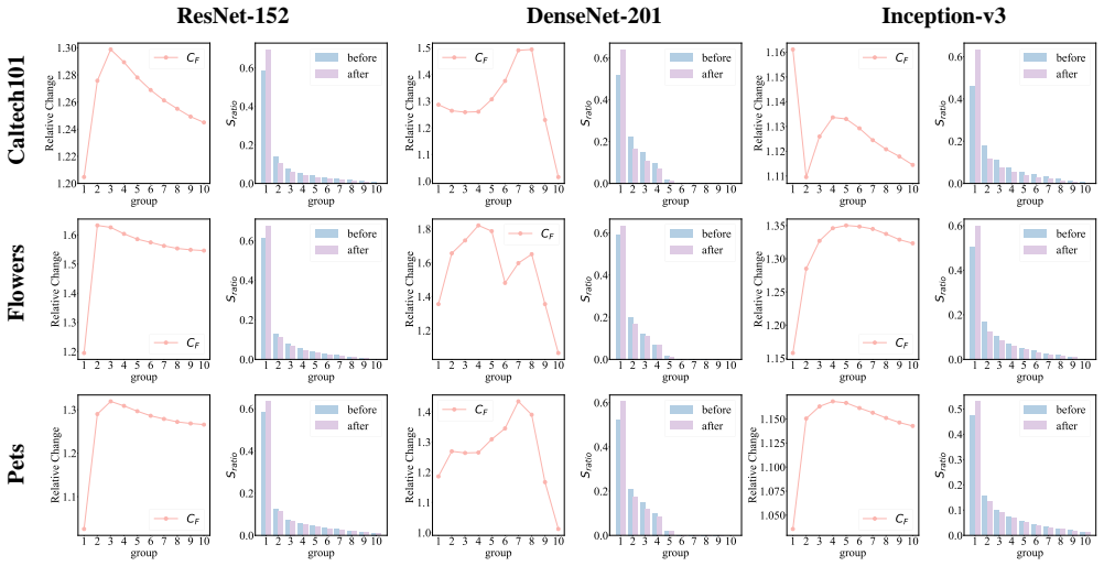
The central claim is that a pre-trained model's transferability to a downstream task is determined by the distribution of spectral components of its extracted features, not by properties of the whole feature set. The paper observes, through SVD of features before and after fine-tuning, that fine-tuning concentrates the singular-value distribution onto components with larger singular values, and that these components transfer better. DISCO formalizes this as $S_{\mathrm{DISCO}} = \sum_{g=1}^{G} S_g^{\mathrm{task}} \cdot S_g^{\mathrm{ratio}}$, with $S_g^{\mathrm{task}}$ measuring how well the $g$-th component separates target classes (nearest-centroid confidence) or fits target regression labels (linear least squares), and $S_g^{\mathrm{ratio}}$ the share of total singular values in that component. The paper reports that this score achieves the highest average weighted Kendall's tau among compared metrics on all three benchmarks.
Load-bearing premise
The paper assumes that the observed tendency of fine-tuning to concentrate singular values onto the largest spectral components, measured on three CNN architectures and three image datasets, is a general property of fine-tuning across architectures, tasks, and domain gaps.
Editorial extensions
If this is right
- Model hubs can be ranked with a single forward pass plus a lightweight classifier, avoiding per-model fine-tuning.
- The same framework works for classification and regression, so object detection and other multi-task settings can share one selection criterion.
- Self-supervised models, which lack pre-trained classifiers, can still be ranked because the score uses only features and target labels.
- With hard-example selection, rankings remain strong at 20 to 40 percent of the data, making the method practical for large target datasets.
- The score is a weighted sum of interpretable per-component terms, so a model's transferability profile can be inspected rather than reduced to a single black-box number.
Reading between the lines
- If the spectral-concentration pattern holds for transformer backbones, DISCO could be applied to large model hubs of foundation models essentially unchanged, since it only needs features and labels.
- The per-component weighting suggests a testable extension: instead of choosing one model, one could blend spectral components across models, selecting the best component per group to form an ensemble.
- The hard-example sampling insight, that hard examples carry more information about transferability, could be reused by other transferability metrics, since the paper shows random sampling loses more accuracy at equal sample sizes.
Editorial analysis
A structured set of objections, weighed in public.
Referee Report
Summary. The paper proposes DISCO, a transferability metric for pre-trained model selection. It performs SVD on features extracted by each candidate model, groups the singular values into spectral components, and scores each component with a task-specific measure (a nearest-centroid classifier score for classification, a linear-regression score for object detection) weighted by the component's singular-value share (Eq. 6, Eq. 10, Eq. 13). The authors motivate the weighting by an empirical observation that fine-tuning concentrates singular values onto larger spectral components (Fig. 2, App. B.1). DISCO is evaluated with weighted Kendall's tau against ground-truth fine-tuning results on 11 classification datasets for supervised and self-supervised CNN pools and on five object detection datasets with six YOLO variants, reporting average tau values of 0.739, 0.726, and 0.634, respectively, and is presented as achieving state-of-the-art model-selection performance.
Significance. If the empirical premise holds, DISCO is a simple, label-based, fine-tuning-free scoring method that extends naturally from classification to regression-style tasks, and the hard-example selection in Sec. 3.4 addresses practical scalability. The paper's strengths are its clean SVD decomposition, the task-specific score design, and the breadth of classification benchmarks, including both supervised and self-supervised model pools. The appendix's extended benchmark and tie-correction analysis are honest additions, but they also expose the main unresolved issue: the load-bearing spectral-concentration premise is verified only on a small set of CNNs and is not checked on transformers where the method's average correlation drops substantially.
major comments (4)
- [3.2, Eq. (6); Fig. 2; App. B.1 and B.5, Table 9] The rating weight Sg_ratio in Eq. (6), which is the only new ingredient distinguishing DISCO from a plain sum of per-component task scores, is justified entirely by the empirical claim that fine-tuning concentrates singular values onto larger spectral components. That claim is demonstrated in Fig. 2 and App. B.1 on exactly three CNN backbones (ResNet-152, DenseNet-201, Inception-v3) and three datasets (Caltech101, Flowers, Pets). The extended benchmark in App. B.5 includes ViT-S, ViT-B, and Swin-T, but it reports only ranking correlations: the average tau drops from 0.739 in Table 1 to 0.554 in Table 9. Because the spectral-concentration diagnostic for transformers is never shown, the premise of Eq. (6) remains unverified outside the CNN family, and a failure of that premise could misrank models even when the per-component task scores are accurate. Please report the CF and Sratio plots for the three transformer models in App. B.5 and provide an ablation on the extended pool that replaces Sg_ratio with uniform weights or with architecture-specific weights.
- [4.1, Tables 1 and 2] The claimed state-of-the-art result is not supported by any uncertainty quantification or significance test. The average advantage over NCTI is only 0.013 on supervised models (0.739 vs. 0.726) and 0.007 on self-supervised models (0.726 vs. 0.719), and the per-dataset signs are mixed: for example, in Table 1 DISCO scores 0.575 on Pets where NCTI scores 0.924, and in Table 2 DISCO scores 0.542 on Pets where NCTI scores 0.805. Since each table entry appears to be a single deterministic computation, a paired bootstrap or permutation test across the 11 datasets would clarify whether the average gain is reliable. Without this, the headline 'state-of-the-art' claim is fragile.
- [4.3, Table 3] The object-detection experiment is too narrow to support the paper's generality claim. The pool consists of six YOLOv5/YOLOv8 variants from the same detector family, all pre-trained on COCO, and the five datasets yield only 15 pairwise comparisons per dataset, making tau values and top-k probabilities coarse. The perfect Pr(top1)=1.000 on this small pool is not strong evidence that the regression score in Eq. (12) generalizes to diverse detection architectures. Please extend the pool to at least one non-YOLO family (e.g., Faster R-CNN or a transformer detector) or temper the claim of generality accordingly.
- [3.4] The complexity statement for naive SVD is incorrect. For a matrix Z in R^{N x d}, standard SVD complexity is O(N d^2) when N > d, not O(N^3 d) as stated. After PCA reduction to d=128 in App. A.2, the relevant tall-skinny regime indeed gives O(N d^2). The empirical runtime results in Fig. 4d and Table 5 may still be valid, but the analytical motivation for hard-example selection should be corrected and re-derived.
minor comments (4)
- [3.2 and 4.4, Fig. 4c] The main experiments use G=10 (Sec. 3.2), but Sec. 4.4 states that G=6 or G=8 'offer the best balance.' Please clarify whether Tables 1-3 use G=10 throughout and whether the reported averages change if the recommended G is used; this affects how the reader interprets the group-number sensitivity.
- [App. B.6, Table 10] The tie-correction analysis considers models within 0.1% accuracy of each other as tied, but it reports only DISCO vs. SFDA and LogME, omitting NCTI and ETran, which are the relevant competitors in Tables 1 and 3. Please include those baselines or explain the omission.
- [Throughout] Several small typographical errors should be fixed, including 'framawork' in the caption of Fig. 4a and 'featrue' in the text surrounding Eq. (16).
- [4.3 and App. B.4, Table 8] The object-detection ground-truth table does not state the training protocol (epochs, batch size, augmentation, hyperparameter sweep) used to obtain the mAP50 values. Adding these details would make the benchmark reproducible.
Circularity Check
No significant circularity: DISCO's score is constructed from pre-fine-tuning SVD components and downstream labels, with fine-tuning performance used only for evaluation.
full rationale
The derivation chain is self-contained. DISCO's score (Eq. 6) is a weighted sum S_DISCO = sum_g S_g_task * S_g_ratio, where S_g_ratio (Eq. 4) is computed from singular values of the original pre-fine-tuning feature matrix Z, and S_g_task is either a nearest-centroid classifier accuracy on the g-th spectral component (Eqs. 7-9) or a negative MSE of a pseudo-inverse linear fit (Eqs. 11-12). No parameter is fitted to the ground-truth fine-tuning accuracies {P^m}; those accuracies enter only in the evaluation protocol (weighted Kendall's tau, Appendix A.1) after the metric has been computed. The empirical observation that fine-tuning concentrates singular values onto larger components (Fig. 2, Appendix B.1) is used as motivation for the S_g_ratio weighting, not as a fitted calibration: the weight is not chosen to optimize tau on the benchmarks. Neither is any load-bearing result imported from the authors' own prior work; the cited sources for fine-tuning ground truth (Shao et al. 2022) and benchmark protocols are external and used for data or evaluation, not to justify the construction. The extended-benchmark and robustness analyses (Tables 9-10) are additional checks, not part of the score definition. The concern that the spectral-concentration premise is validated on only three CNNs and three datasets is a generality or robustness limitation, not a circularity: it does not make Eq. 6 equivalent to its inputs by construction. Therefore no circular step is present.
Assumptions & free parameters
free parameters (2)
- G (number of spectral groups) =
10 in main experiments; 6 or 8 reported as better in Figure 4c
- PCA dimension for features =
128
assumptions (3)
- domain assumption Empirical generalization: after fine-tuning, singular values concentrate on components with larger singular values, and these components are more transferable.
- domain assumption Multivariate Gaussian class-conditional distributions for features within each spectral component.
- domain assumption Linear or least-squares fit of features to labels is a sufficient proxy for fine-tuned regression performance.
Cite this review
Pith. "Pith review of Assessing Pre-Trained Models for Transfer Learning Through Distribution of Spectral Components." pith.science (2026). https://pith.science/paper/H7WWLXUP
@misc{pith2026241219085,
  author       = {Pith},
  title        = {Pith review of: Assessing Pre-Trained Models for Transfer Learning Through Distribution of Spectral Components},
  year         = {2026},
  howpublished = {\url{https://pith.science/paper/H7WWLXUP}},
  note         = {Machine review of arXiv:2412.19085}
}
read the original abstract
Pre-trained model assessment for transfer learning aims to identify the optimal candidate for the downstream tasks from a model hub, without the need of time-consuming fine-tuning. Existing advanced works mainly focus on analyzing the intrinsic characteristics of the entire features extracted by each pre-trained model or how well such features fit the target labels. This paper proposes a novel perspective for pre-trained model assessment through the Distribution of Spectral Components (DISCO). Through singular value decomposition of features extracted from pre-trained models, we investigate different spectral components and observe that they possess distinct transferability, contributing diversely to the fine-tuning performance. Inspired by this, we propose an assessment method based on the distribution of spectral components which measures the proportions of their corresponding singular values. Pre-trained models with features concentrating on more transferable components are regarded as better choices for transfer learning. We further leverage the labels of downstream data to better estimate the transferability of each spectral component and derive the final assessment criterion. Our proposed method is flexible and can be applied to both classification and regression tasks. We conducted comprehensive experiments across three benchmarks and two tasks including image classification and object detection, demonstrating that our method achieves state-of-the-art performance in choosing proper pre-trained models from the model hub for transfer learning.
Figures


Figures from the paper (2 more)

Reference graph
Works this paper leans on
-
[1]
S.; Davis, A.; Dean, J.; Devin, M.; et al
Abadi, M.; Agarwal, A.; Barham, P.; Brevdo, E.; Chen, Z.; Citro, C.; Corrado, G. S.; Davis, A.; Dean, J.; Devin, M.; et al. 2016. Tensorflow: Large-scale machine learning on heterogeneous distributed systems. arXiv preprint arXiv:1603.04467
arXiv 2016
-
[2]
M.; Rupprecht, C.; and Vedaldi, A
Asano, Y. M.; Rupprecht, C.; and Vedaldi, A. 2019. Self-labelling via simultaneous clustering and representation learning. arXiv preprint arXiv:1911.05371
arXiv 2019
-
[3]
ASD. 2022. wlots Dataset. \ https://universe.roboflow.com/asd-culfr/wlots . Accessed: 2023-01-27
work page 2022
-
[4]
Bolya, D.; Mittapalli, R.; and Hoffman, J. 2021. Scalable diverse model selection for accessible transfer learning. In NeurIPS
work page 2021
-
[5]
Bossard, L.; Guillaumin, M.; and Van Gool, L. 2014. Food-101--mining discriminative components with random forests. In ECCV
work page 2014
-
[6]
D.; Dhariwal, P.; Neelakantan, A.; Shyam, P.; Sastry, G.; Askell, A.; et al
Brown, T.; Mann, B.; Ryder, N.; Subbiah, M.; Kaplan, J. D.; Dhariwal, P.; Neelakantan, A.; Shyam, P.; Sastry, G.; Askell, A.; et al. 2020. Language models are few-shot learners. In NeurIPS
work page 2020
-
[7]
Caron, M.; Bojanowski, P.; Joulin, A.; and Douze, M. 2018. Deep clustering for unsupervised learning of visual features. In ECCV
work page 2018
-
[8]
Caron, M.; Misra, I.; Mairal, J.; Goyal, P.; Bojanowski, P.; and Joulin, A. 2020. Unsupervised learning of visual features by contrasting cluster assignments. In NeurIPS
work page 2020
Show all 62 references
-
[9]
Chen, X.; Fan, H.; Girshick, R.; and He, K. 2020. Improved baselines with momentum contrastive learning. arXiv preprint arXiv:2003.04297
2020 arXiv
-
[10]
Cimpoi, M.; Maji, S.; Kokkinos, I.; Mohamed, S.; and Vedaldi, A. 2014. Describing textures in the wild. In CVPR
2014
-
[11]
Dettmers, T.; Pagnoni, A.; Holtzman, A.; and Zettlemoyer, L. 2024. Qlora: Efficient finetuning of quantized llms. In NeurIPS
2024
-
[12]
Devlin, J.; Chang, M.-W.; Lee, K.; and Toutanova, K. 2018. Bert: Pre-training of deep bidirectional transformers for language understanding. arXiv preprint arXiv:1810.04805
2018 arXiv
-
[13]
Ding, N.; Chen, X.; Levinboim, T.; Changpinyo, S.; and Soricut, R. 2022. Pactran: Pac-bayesian metrics for estimating the transferability of pretrained models to classification tasks. In ECCV
2022
-
[14]
Ding, Y.; Jiang, B.; Yu, A.; Zheng, A.; and Liang, J. 2024. Which Model to Transfer? A Survey on Transferability Estimation. arXiv preprint arXiv:2402.15231
2024 arXiv
-
[15]
Donahue, J.; Jia, Y.; Vinyals, O.; Hoffman, J.; Zhang, N.; Tzeng, E.; and Darrell, T. 2014. Decaf: A deep convolutional activation feature for generic visual recognition. In ICML
2014
-
[16]
Dosovitskiy, A.; Beyer, L.; Kolesnikov, A.; Weissenborn, D.; Zhai, X.; Unterthiner, T.; Dehghani, M.; Minderer, M.; Heigold, G.; Gelly, S.; et al. 2020. An image is worth 16x16 words: Transformers for image recognition at scale. arXiv preprint arXiv:2010.11929
2020 arXiv
-
[17]
Erhan, D.; Courville, A.; Bengio, Y.; and Vincent, P. 2010. Why does unsupervised pre-training help deep learning? In AISTATS
2010
-
[18]
K.; Winn, J.; and Zisserman, A
Everingham, M.; Van Gool, L.; Williams, C. K.; Winn, J.; and Zisserman, A. 2010. The pascal visual object classes (voc) challenge. IJCV, 88: 303--338
2010
-
[19]
Fei-Fei, L.; Fergus, R.; and Perona, P. 2004. Learning generative visual models from few training examples: An incremental bayesian approach tested on 101 object categories. In CVPR
2004
-
[20]
Gholami, M.; Akbari, M.; Wang, X.; Kamranian, B.; and Zhang, Y. 2023. Etran: Energy-based transferability estimation. In ICCV
2023
-
[21]
Grill, J.-B.; Strub, F.; Altch \'e , F.; Tallec, C.; Richemond, P.; Buchatskaya, E.; Doersch, C.; Avila Pires, B.; Guo, Z.; Gheshlaghi Azar, M.; et al. 2020. Bootstrap your own latent-a new approach to self-supervised learning. In NeurIPS
2020
-
[22]
He, K.; Fan, H.; Wu, Y.; Xie, S.; and Girshick, R. 2020. Momentum contrast for unsupervised visual representation learning. In CVPR
2020
-
[23]
He, K.; Zhang, X.; Ren, S.; and Sun, J. 2016. Deep residual learning for image recognition. In CVPR
2016
-
[24]
home. 2022. NFL-competition Dataset. \ https://universe.roboflow.com/home-mxzv1/nfl-competition . Accessed: 2023-01-18
2022
-
[25]
Huang, G.; Liu, Z.; Van Der Maaten, L.; and Weinberger, K. Q. 2017. Densely connected convolutional networks. In CVPR
2017
-
[26]
Jia, M.; Tang, L.; Chen, B.-C.; Cardie, C.; Belongie, S.; Hariharan, B.; and Lim, S.-N. 2022. Visual prompt tuning. In ECCV
2022
-
[27]
Jocher, G.; Chaurasia, A.; and Qiu, J. 2023. YOLO by Ultralytics
2023
-
[28]
Jocher, G.; et al. 2023. YOLOv5 by Ultralytics. 2020. URL https://github. com/ultralytics/yolov5
2023
-
[29]
Krause, J.; Deng, J.; Stark, M.; and Fei-Fei, L. 2013. Collecting a large-scale dataset of fine-grained cars
2013
-
[30]
Krizhevsky, A.; Hinton, G.; et al. 2009. Learning multiple layers of features from tiny images
2009
-
[31]
Kumar, A.; Raghunathan, A.; Jones, R.; Ma, T.; and Liang, P. 2022. Fine-tuning can distort pretrained features and underperform out-of-distribution. arXiv preprint arXiv:2202.10054
2022 arXiv
-
[32]
Li, J.; Zhou, P.; Xiong, C.; and Hoi, S. C. 2020. Prototypical contrastive learning of unsupervised representations. arXiv preprint arXiv:2005.04966
2020 arXiv
-
[33]
Li, X.; Hu, Z.; Ge, Y.; Shan, Y.; and Duan, L.-Y. 2023. Exploring model transferability through the lens of potential energy. In ICCV
2023
-
[34]
Li, Y.; Jia, X.; Sang, R.; Zhu, Y.; Green, B.; Wang, L.; and Gong, B. 2021. Ranking Neural Checkpoints. In CVPR
2021
-
[35]
Lin, T.-Y.; Maire, M.; Belongie, S.; Hays, J.; Perona, P.; Ramanan, D.; Doll \'a r, P.; and Zitnick, C. L. 2014. Microsoft coco: Common objects in context. In ECCV
2014
-
[36]
Liu, X.; Zheng, Y.; Du, Z.; Ding, M.; Qian, Y.; Yang, Z.; and Tang, J. 2023. GPT understands, too. AI Open
2023
-
[37]
Magonis, D. 2022. valorant Dataset. \ https://universe.roboflow.com/daniels-magonis-0pjzx/valorant-9ufcp . Accessed: 2023-01-27
2022
-
[38]
Maji, S.; Rahtu, E.; Kannala, J.; Blaschko, M.; and Vedaldi, A. 2013. Fine-grained visual classification of aircraft. arXiv preprint arXiv:1306.5151
2013 arXiv
-
[39]
Nguyen, C.; Hassner, T.; Seeger, M.; and Archambeau, C. 2020. Leep: A new measure to evaluate transferability of learned representations. In ICML
2020
-
[40]
Nilsback, M.-E.; and Zisserman, A. 2008. Automated flower classification over a large number of classes. In 2008 Sixth Indian conference on computer vision, graphics & image processing. IEEE
2008
-
[41]
P \'a ndy, M.; Agostinelli, A.; Uijlings, J.; Ferrari, V.; and Mensink, T. 2022. Transferability estimation using bhattacharyya class separability. In CVPR
2022
-
[42]
M.; Vedaldi, A.; Zisserman, A.; and Jawahar, C
Parkhi, O. M.; Vedaldi, A.; Zisserman, A.; and Jawahar, C. 2012. Cats and dogs. In CVPR
2012
-
[43]
W.; Hallacy, C.; Ramesh, A.; Goh, G.; Agarwal, S.; Sastry, G.; Askell, A.; Mishkin, P.; Clark, J.; et al
Radford, A.; Kim, J. W.; Hallacy, C.; Ramesh, A.; Goh, G.; Agarwal, S.; Sastry, G.; Askell, A.; Mishkin, P.; Clark, J.; et al. 2021. Learning transferable visual models from natural language supervision. In ICML
2021
-
[44]
Roboflow, T. 2022. Blood Cell Detection Dataset. \ https://universe.roboflow.com/team-roboflow/blood-cell-detection-1ekwu . Accessed: 2023-01-18
2022
-
[45]
Russakovsky, O.; Deng, J.; Su, H.; Krause, J.; Satheesh, S.; Ma, S.; Huang, Z.; Karpathy, A.; Khosla, A.; Bernstein, M.; et al. 2015. Imagenet large scale visual recognition challenge. IJCV, 115: 211--252
2015
-
[46]
Sandler, M.; Howard, A.; Zhu, M.; Zhmoginov, A.; and Chen, L.-C. 2018. Mobilenetv2: Inverted residuals and linear bottlenecks. In CVPR
2018
-
[47]
Shao, W.; Zhao, X.; Ge, Y.; Zhang, Z.; Yang, L.; Wang, X.; Shan, Y.; and Luo, P. 2022. Not all models are equal: Predicting model transferability in a self-challenging fisher space. In ECCV
2022
-
[48]
Szegedy, C.; Liu, W.; Jia, Y.; Sermanet, P.; Reed, S.; Anguelov, D.; Erhan, D.; Vanhoucke, V.; and Rabinovich, A. 2015. Going deeper with convolutions. In CVPR
2015
-
[49]
Szegedy, C.; Vanhoucke, V.; Ioffe, S.; Shlens, J.; and Wojna, Z. 2016. Rethinking the inception architecture for computer vision. In CVPR
2016
-
[50]
Tan, M.; Chen, B.; Pang, R.; Vasudevan, V.; Sandler, M.; Howard, A.; and Le, Q. V. 2019. Mnasnet: Platform-aware neural architecture search for mobile. In CVPR
2019
-
[51]
Tian, Y.; Sun, C.; Poole, B.; Krishnan, D.; Schmid, C.; and Isola, P. 2020. What makes for good views for contrastive learning? In NeurIPS
2020
-
[52]
T.; Nguyen, C
Tran, A. T.; Nguyen, C. V.; and Hassner, T. 2019. Transferability and hardness of supervised classification tasks. In ICCV
2019
-
[53]
Traore, M. 2022. Forklift Dataset. \ https://universe.roboflow.com/mohamed-traore-2ekkp/forklift-dsitv . Accessed: 2023-01-15
2022
-
[54]
Wang, Z.; Luo, Y.; Zheng, L.; Huang, Z.; and Baktashmotlagh, M. 2023. How far pre-trained models are from neural collapse on the target dataset informs their transferability. In ICCV
2023
-
[55]
Wolf, T.; Debut, L.; Sanh, V.; Chaumond, J.; Delangue, C.; Moi, A.; Cistac, P.; Rault, T.; Louf, R.; Funtowicz, M.; et al. 2019. Huggingface's transformers: State-of-the-art natural language processing. arXiv preprint arXiv:1910.03771
2019 arXiv
-
[56]
X.; and Lin, D
Wu, Z.; Xiong, Y.; Yu, S. X.; and Lin, D. 2018. Unsupervised feature learning via non-parametric instance discrimination. In CVPR
2018
-
[57]
A.; Oliva, A.; and Torralba, A
Xiao, J.; Hays, J.; Ehinger, K. A.; Oliva, A.; and Torralba, A. 2010. Sun database: Large-scale scene recognition from abbey to zoo. In 2010 IEEE computer society conference on computer vision and pattern recognition
2010
-
[58]
Xu, H.; and Kang, U. 2023. Fast and accurate transferability measurement by evaluating intra-class feature variance. In ICCV
2023
-
[59]
Yosinski, J.; Clune, J.; Bengio, Y.; and Lipson, H. 2014. How transferable are features in deep neural networks? In NeurIPS
2014
-
[60]
You, K.; Liu, Y.; Wang, J.; and Long, M. 2021. Logme: Practical assessment of pre-trained models for transfer learning. In ICML
2021
-
[61]
, " * write output.state after.block = add.period write newline
ENTRY address archivePrefix author booktitle chapter edition editor eid eprint howpublished institution isbn journal key month note number organization pages publisher school series title type volume year label extra.label sort.label short.list INTEGERS output.state before.all...
-
[62]
write newline
" write newline "" before.all 'output.state := FUNCTION n.dashify 't := "" t empty not t #1 #1 substring "-" = t #1 #2 substring "--" = not "--" * t #2 global.max substring 't := t #1 #1 substring "-" = "-" * t #2 global.max substring 't := while if t #1 #1 substring * t #2 gl...
Reviewed August 11, 2026 · model on record in the stance chip above.
Discussion (0). Continue with ORCID to comment.