REVIEW 4 major objections 5 minor 61 references
Automated Architecture Design for Deep Neural Networks
T0 review · 4 major / 5 minor · reviewed 2026-08-14 · deepseek-v4-flash
Pith's one-line read Automated forward thinking builds MNIST classifiers layer by layer from a candidate pool, reaching about 97.5 percent test accuracy—slightly better than every multilayer perceptron the thesis tested.
desk verdict A genuinely new but very preliminary constructive algorithm; the head-to-head MNIST claim collapses once you notice the baselines were selected on the test set, so treat it as an idea worth testing, not a result. read the letter →
The pith
A machine-rendered reading of the paper's core claim, the machinery that carries it, and where it could break.
The reading
What carries the argument
The mechanism is a candidate-pool layer selector grafted onto forward thinking. Forward thinking is a greedy training scheme that adds one hidden layer at a time: the new layer is trained on the network's current output, its input weights are frozen, and the output layer is discarded and retrained, so error never has to flow through more than one fresh layer. Automated forward thinking adds a search step: a pool of eight candidate layers, each a random width between 50 and 1000 in multiples of 50, is trained for two epochs, and the candidate with the best validation accuracy is the one inserted. A stricter stopping rule—or equivalently, training extra layers and then picking the layer count with the best accuracy-versus-complexity trade-off—keeps the final network small. This machinery carries the argument because it converts architecture selection from a human hyperparameter choice into a local, greedy, randomized search over layer widths.
What would settle it
Re-run the random and evolutionary searches exactly as described but choose architectures using a held-out validation set, never touching the 10,000-example test set until the final selected model is evaluated; if the best fully trained baselines then reach or exceed the 97.54 percent average of automated forward thinking on the same test split, the claim that automated forward thinking outperforms all tested MLPs is falsified.
Extended reading notes
Core claim
The discovery is an algorithm, named automated forward thinking, that turns the greedy layer-wise training idea of forward thinking into a complete architecture search. Starting from the input, the algorithm keeps a pool of eight candidate hidden layers whose widths are drawn uniformly from 50 to 1000 in steps of 50; each candidate is trained for two epochs, the one with the highest validation accuracy is inserted into the network, its input weights are frozen, the output layer is retrained, and the process repeats. Across 20 runs on MNIST this produced networks with an average test accuracy of 97.54 percent and a standard deviation of 0.17 percent, with the best architecture [900, 600, 600, 300] reaching 97.86 percent. The thesis concludes that automated forward thinking builds deeper networks than the standard two-hidden-layer MLPs found by manual, random, and evolutionary search, and that it yields better test performance than any MLP investigated in the thesis.
Load-bearing premise
The comparison treats the reported test accuracies as unbiased measures of generalization, but the random and evolutionary baselines chose architectures using the test set itself, so those baselines can only look better than a clean validation protocol would make them; if that bias is corrected, automated forward thinking's margin may disappear.
Editorial extensions
If this is right
- If the central claim holds, deep feedforward networks can be constructed layer by layer with no backpropagation through the full stack, which removes the vanishing-gradient obstacle that usually limits depth.
- On MNIST, a fully automated construction rule reaches about 97.5 percent test accuracy—slightly better than the best manually designed or searched multilayer perceptrons—suggesting that human architecture expertise buys little on this task once a good greedy selector is in place.
- The small standard deviation of 0.17 percent across runs means the improvement over the 97.3 percent baselines, though modest, is consistent rather than the product of a single lucky run.
- Because the selection criterion is validation accuracy, automated forward thinking also supplies a natural early-stopping rule for depth, which can be tuned against model size.
- The same layer-by-layer construction can be stopped after any number of layers, so the algorithm produces a family of architectures of increasing depth and lets the user choose the point where added complexity stops paying for itself.
Reading between the lines
- The candidate-pool layer selector is a general constructive search primitive; the same pool-and-select step could be applied to convolutional filters, recurrent cells, or residual blocks and tested on other data sets, though the thesis only demonstrates feedforward MLPs on MNIST.
- The paper's baseline comparisons are biased in favor of random and evolutionary search: both selected architectures using test-set accuracy, so a validation-only rerun could shrink or erase the roughly 0.2-percentage-point margin over the best MLPs.
- The post-hoc layer-count selection is essentially a complexity-penalized model selection rule; formalizing it as accepting a layer only when validation loss improves by at least a specified margin would turn the heuristic into a stopping rule with a sharper complexity guarantee.
- If the margin over baselines survives a clean validation protocol, the practical consequence is that architecture search for feedforward networks can be run on a single GPU in minutes rather than requiring large parallel search farms.
Signed reviews
Editorial analysis
A structured set of objections, weighed in public.
Referee Report
Summary. The manuscript, a bachelor thesis posted to arXiv, studies automated architecture design for feedforward neural networks. It surveys neural architecture search and constructive dynamic learning, then presents empirical comparisons on MNIST among manual search, random search, evolutionary search, several cascade-correlation variants (Cascor, Caser, CaserRe), forward thinking, and the author's proposed Automated Forward Thinking (AFT). AFT greedily adds hidden layers selected from a candidate pool of eight randomly sized layers, training each candidate for two epochs and choosing the one with highest validation accuracy. The paper reports that AFT builds deeper networks than the MLP baselines and achieves an average test accuracy of 97.54% (std 0.17%), with the best architecture [900,600,600,300] reaching 97.86%, and concludes that AFT outperforms every MLP investigated. The central empirical claim is currently undermined by the documented use of the test set during random and evolutionary search and by best-of-20 selection for the AFT headline number.
Significance. If the comparison were clean, the contribution would be a useful, simple constructive NAS method: AFT avoids end-to-end backpropagation through deep stacks, produces interpretable layer-by-layer training curves, and is cheap enough to run 20 times on a modest GPU. The paper also gives a clear negative result for cascade-correlation on high-dimensional MNIST and an interesting fix, CaserRe, which reuses output weights to reduce performance dips. Its strengths are the explicit protocol statement in Section 4.1.2, which makes the later violation easy to identify, the candid acknowledgment of the preliminary scope, and the transparent reporting of standard deviations. However, as written, the headline comparison is not trustworthy: the baselines are test-selected, the AFT best is a post-hoc test-set choice, and there is no statistical test. The contribution may be salvageable with a corrected protocol and additional benchmark tasks, but the current evidence is not sufficient to support the central claim.
major comments (4)
- [§4.2.2, §4.2.3, §4.1.2] The central comparison is invalidated by test-set leakage in the two search baselines. Section 4.1.2 states that the testing set will not be used until the final model architecture is decided on and that all model decisions will be based on validation and training data, yet Section 4.2.2 says random-search networks "will be assessed on the training set and the testing set" after training, and Section 4.2.3 defines evolutionary fitness as "the accuracy of the network on the testing set after training for three epochs." The reported best random and evolutionary architectures (Tables 2, 4, 6) were therefore selected partly on test accuracy, making their 97.2–97.3% test figures optimistically biased estimates of generalization. Automated forward thinking, by contrast, selects candidate layers on validation accuracy (Section 4.3.3). Comparing a test-selected baseline with a validation-selected construction inflates the apparent advantage of AFT. The random and evolutionary searches should be re-run with all selection decisions made on the validation set, the test set held out until one final architecture per method is evaluated, and the comparison repeated with a corrected protocol.
- [§4.3.3, Table 9] The headline AFT result is a best-of-20 test-set choice, not a clean out-of-sample estimate. The text reports that the "best performing network architecture is [900, 600, 600, 300] with a testing accuracy of 97.86%" after running the algorithm 20 times; Table 9 lists the ten smallest architectures with their Test Acc values, and the runs appear to be scored on the test set. Selecting the best of 20 architectures by test accuracy is itself a form of test-set model selection, and it will overestimate the performance a user would obtain by running AFT once and deploying the result. The average AFT test accuracy (97.54% ± 0.17%) is a more meaningful statistic, but even that average is not compared statistically with the baselines, and it overlaps with the baseline means once the baselines' selection bias is accounted for. The authors should pre-register a single architecture choice, or select the architecture on validation and evaluate it once on test, and should provide a paired or corrected significance comparison.
- [§4.1.2, §4.4] The claim that AFT "yields better performance on the test data than any MLP investigated in this thesis" rests on a single dataset (MNIST), one run each of the random and evolutionary search procedures, and no significance tests. Section 4.1.2 explicitly restricts the benchmark to MNIST, and Section 4.1 acknowledges that the results "will not be sufficient to confirm or reject any hypotheses"; Section 4.4 similarly calls the evidence preliminary. A single-dataset comparison with one realization of two baseline families cannot support a general superiority claim, especially when the reported differences are on the order of 0.2–0.3 percentage points. The manuscript should either restrict the conclusion to "on MNIST under a corrected protocol, AFT performed comparably or slightly better" or add additional benchmark tasks and multiple repeats of every search algorithm with validation-based selection.
- [§4.3.3, §4.3.4] The "fully automated" characterization is overstated. The AFT algorithm requires the user to set the candidate-pool size (8), the number of training epochs per candidate (2), the layer-width interval [50, 1000] in multiples of 50, the early-stopping patience, and, most restrictively, the constraint that layer widths must be subsequently decreasing, a choice the author says will be "ommit[ted]" from discussion. Section 4.3.4 acknowledges that bounds on hidden-layer widths are needed. These hyperparameters are hand-tuned with no sensitivity analysis, and the decreasing-width constraint is a substantial inductive bias that excludes many architectures. The paper should report sensitivity to these choices or reduce the automaticity claim accordingly.
minor comments (5)
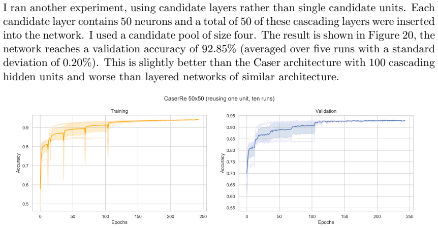
- [§4.2.2, Table 1, §4.2.3] There are numerical inconsistencies: the text in Section 4.2.2 says each sampled network is trained for five epochs, while the caption of Table 1 says three epochs; Section 4.2.2 says 100 configurations are sampled, but Section 4.2.3 says random search picked 200 networks. Please reconcile these numbers.
- [§4.2.2, §4.3.2, Table 9] The paper alternates between validation accuracy, test accuracy, and testing accuracy without a consistent definition. For example, Section 4.3.2 Table 7 reports Validation Accuracy, while Section 4.3.4 discusses testing accuracy, and the columns labeled Test Acc in Table 9 are produced by a procedure that Section 4.3.3 describes as validation-based. This makes it hard to audit which data was used for each decision.
- [Figure 9] Figure 9 is described as an animation, but in the PDF it is a static plot; either embed a playable animation or change the description to a static exploration plot.
- [§3.1, §4.3.3, §4.3.4] There are several typos and small errors, including "constant form of constant estimation" (Section 3.1), "ommit" (Section 4.3.3), and "algortihms" (Section 4.3.4). A careful proofread is recommended.
- [§4.2.1] The manual-search baseline is a single network trained without dropout, but the Keras example it is based on uses dropout and reports 98.40%; please state explicitly that this baseline is intended as a no-regularization reference and not as a state-of-the-art comparison.
Circularity Check
Comparison is partly circular: random and evolutionary baselines are selected on the test set, and the headline AFT accuracy is a best-of-20 test-set choice.
-
fitted input called prediction
[Section 4.2.3 (Evolutionary Search), fitness definition; relied on in Section 4.4]
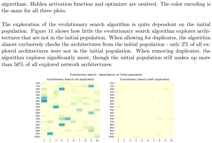
"The fitness is just the accuracy of the network on the testing set after training for three epochs. As was done in random search, each network is trained three times. The average test accuracy after three epochs is taken as the network's fitness."
The evolutionary baselines are chosen to maximize test-set accuracy, and their reported final test accuracies are then used as evidence of their generalization. The selection metric and the reported evaluation metric are the same quantity, so the baseline numbers are fitted values rather than independent estimates. Section 4.4 uses them to conclude that automated forward thinking 'yields better performance on the test data than any MLP investigated,' but AFT layers are selected on validation accuracy (Section 4.3.3), so the comparison is between a test-fitted baseline and a validation-fitted method, inflating the apparent advantage.
-
fitted input called prediction
[Section 4.2.2 (Random Search), initial assessment protocol]
"The program will randomly sample 100 configurations from the search space. Each of the sampled networks will be trained on the training data for five epochs and the performance will be assessed on the training set and the testing set."
This contradicts the paper's own protocol in Section 4.1.2 that 'The testing set will not be used until the final model architecture is decided on.' The random-search candidates selected for full training and final reporting are exposed to the test set during the search, so their reported test accuracies are partly fitted to the test metric. This biases the baseline comparison in the same direction as the evolutionary search step.
1 more flagged steps
-
fitted input called prediction
[Section 4.3.3 (Automated Forward Thinking), Table 9 and following text]
"Across 20 runs of the algorithm, the average test accuracy is 97.54% (with a standard deviation of only 0.17%) - which is better than any other algorithm I have investigated in this thesis. Half of the architectures use below five layers, the other half uses five or more layers. The best performing network architecture is [900, 600, 600, 300] with a testing accuracy of 97.86%."
The headline 'best performing network architecture' is the maximum of 20 test-set evaluations, so 97.86% is a selected statistic rather than an unbiased estimate of the algorithm's generalization. Highlighting this test-selected best as the algorithm's result is a further use of the evaluation metric as a model-selection criterion, though the reported average of 97.54% is a less biased summary.
full rationale
There is no equation-level circularity and no load-bearing self-citation chain; the proposed AFT algorithm is a new constructive procedure whose average test accuracy is not defined by its inputs. The circularity burden lies in the empirical comparison. Section 4.1.2 promises that 'The testing set will not be used until the final model architecture is decided on,' but Section 4.2.3 defines evolutionary fitness as test-set accuracy, and Section 4.2.2 assesses random-search candidates on the testing set. The baselines' reported test accuracies are therefore partly fitted to the same metric used for the final comparison, making the claim that AFT outperforms all investigated MLPs partially circular. In addition, the paper highlights a best-of-20 test-set architecture as its best result. Because the central algorithm itself is validated by an average over runs and the baseline leakage is a protocol flaw rather than a definitional equivalence, the circularity is partial, not total. Correctness risk (invalid baseline protocol) is separate from circularity but is the reason the comparison cannot be taken at face value.
Assumptions & free parameters
free parameters (7)
- Search space bounds (random/evolutionary) =
hidden units 100-1000 in multiples of 50; layers 1-10; activation in {relu, tanh}; optimizer in {SGD, RMSProp}
- Evolutionary algorithm hyperparameters =
population size 50, mutation chance 10%, retain rate 40%, random selection rate 10%
- Candidate pool size (Cascor/Caser/AFT) =
8, 16, 4, and 8 in automated forward thinking
- Candidate training epochs =
1 or 2 epochs
- Layer width range (AFT) =
50 to 1000 in multiples of 50
- Early stopping patience =
2 or 3 epochs without validation improvement
- CaserRe weight reuse threshold =
5% validation accuracy decrease
assumptions (3)
- domain assumption Validation accuracy is a reliable proxy for test accuracy during architecture selection.
- domain assumption Greedy layer-by-layer training can yield competitive final accuracy compared with end-to-end backpropagation.
- domain assumption MNIST is representative enough to draw preliminary conclusions about automated architecture design for feedforward networks.
Cite this review
Pith. "Pith review of Automated Architecture Design for Deep Neural Networks." pith.science (2026). https://pith.science/paper/HCOGVHCL
@misc{pith2026190810714,
  author       = {Pith},
  title        = {Pith review of: Automated Architecture Design for Deep Neural Networks},
  year         = {2026},
  howpublished = {\url{https://pith.science/paper/HCOGVHCL}},
  note         = {Machine review of arXiv:1908.10714}
}
read the original abstract
Machine learning has made tremendous progress in recent years and received large amounts of public attention. Though we are still far from designing a full artificially intelligent agent, machine learning has brought us many applications in which computers solve human learning tasks remarkably well. Much of this progress comes from a recent trend within machine learning, called deep learning. Deep learning models are responsible for many state-of-the-art applications of machine learning. Despite their success, deep learning models are hard to train, very difficult to understand, and often times so complex that training is only possible on very large GPU clusters. Lots of work has been done on enabling neural networks to learn efficiently. However, the design and architecture of such neural networks is often done manually through trial and error and expert knowledge. This thesis inspects different approaches, existing and novel, to automate the design of deep feedforward neural networks in an attempt to create less complex models with good performance that take away the burden of deciding on an architecture and make it more efficient to design and train such deep networks.
Figures

Figures from the paper (23 more)








Reference graph
Works this paper leans on
-
[1]
Bartlett, P. L., Maiorov, V., and Meir, R. (1999). Almost Linear VC Dimension Bounds for Piecewise Polynomial Networks . In Kearns, M. J., Solla, S. A., and Cohn, D. A., editors, Advances in Neural Information Processing Systems 11 , pages 190--196. MIT Press
work page 1999
-
[2]
Bergstra, J. and Bengio, Y. (2012). Random Search for Hyper-Parameter Optimization . The Journal of Machine Learning Research , 13(Feb):281--305
work page 2012
-
[3]
Bianchini, M. and Scarselli, F. (2014). On the Complexity of Shallow and Deep Neural Network Cassifiers . In European Symposium on Artificial Neural Networks , volume 22, pages 371--376
work page 2014
-
[4]
Choromanska, A., Henaff, M., Mathieu, M., Arous, G. B., and LeCun, Y. (2015). The Loss Surfaces of Multilayer Networks . In Proceedings of the 18th International Conference on Artificial Intelligence and Statistics , volume 38 of JMLR: W&CP , pages 192--204. JMLR.org
work page 2015
-
[5]
Conneau, A., Schwenk, H., Barrault, L., and Lecun, Y. (2016). Very Deep Convolutional Networks for Text Classification . arXiv preprint arXiv:1606.01781
arXiv 2016
-
[6]
Cortes, C., Gonzalvo, X., Kuznetsov, V., Mohri, M., and Yang, S. (2017). Adanet: Adaptive Structural Learning of Artificial Neural Networks . In Proceedings of the 34th International Conference on Machine Learning , volume 70, pages 874--883. JMLR
work page 2017
-
[7]
Eldan, R. and Shamir, O. (2016). The Power of Depth for Feedforward Neural Networks . In Conference on Learning Theory , volume 49, pages 907--940
work page 2016
-
[8]
Elsken, T., Metzen, J. H., and Hutter, F. (2019). Neural Architecture Search: A Survey . The Journal of Machine Learning Research , 20(55):1--21
work page 2019
Show all 61 references
-
[9]
Fahlman, S. E. (1991). The Recurrent Cascade-Correlation Architecture . In Lippmann, R. P., Moody, J. E., and Touretzky, D. S., editors, Advances in Neural Information Processing Systems 3 , pages 190--196. Morgan-Kaufmann
1991
-
[10]
Fahlman, S. E. and Lebiere, C. (1990). The Cascade-Correlation Learning Architecture . In Touretzky, D. S., editor, Advances in Neural Information Processing Systems 2 , pages 524--532. Morgan-Kaufmann
1990
-
[11]
Frean, M. (1990). The Upstart Algorithm: A Method for Constructing and Training Feedforward Neural Networks . Neural Computation , 2(2):198--209
1990
-
[12]
Goodfellow, I., Bengio, Y., and Courville, A. (2016). Deep Learning . MIT press
2016
-
[13]
Hanson, S. J. (1990). Meiosis Networks . In Touretzky, D. S., editor, Advances in Neural Information Processing Systems 2 , pages 533--541. Morgan-Kaufmann
1990
-
[14]
Harvey, M. (2017). Let’s evolve a neural network with a genetic algorithm — code included
2017
-
[15]
G., and Wolff, G
Hassibi, B., Stork, D. G., and Wolff, G. (1994). Optimal Brain Surgeon: Extensions and Performance Comparisons . In Cowan, J. D., Tesauro, G., and Alspector, J., editors, Advances in Neural Information Processing Systems 6 , pages 263--270. Morgan-Kaufmann
1994
-
[16]
G., and Wolff, G
Hassibi, B., Stork, D. G., and Wolff, G. J. (1993). Optimal brain surgeon and general network pruning. In IEEE International Conference on Neural Networks , volume 1, pages 293--299. IEEE
1993
-
[17]
He, K., Zhang, X., Ren, S., and Sun, J. (2016). Deep Residual Learning for Image Recognition . In Proceedings of the IEEE Conference on Computer Vision and Pattern Recognition , volume 1, pages 770--778
2016
-
[18]
Hettinger, C., Christensen, T., Ehlert, B., Humpherys, J., Jarvis, T., and Wade, S. (2017). Forward Thinking: Building and Training Neural Networks One Layer at a Time . arXiv preprint arXiv:1706.02480
2017 arXiv
-
[19]
Hinton, G. E. (2012). A Practical Guide to Training Restricted Boltzmann Machines . In Neural Networks: Tricks of the Trade , pages 599--619. Springer
2012
-
[20]
Hornik, K., Stinchcombe, M., and White, H. (1989). Multilayer Feedforward Networks Are Universal Approximators . Neural Networks , 2(5):359--366
1989
-
[21]
Simple Deep Neural Network on the MNIST Dataset
Keras (2019). Simple Deep Neural Network on the MNIST Dataset
2019
-
[22]
Krizhevsky, A., Sutskever, I., and Hinton, G. E. (2017). ImageNet Classification with Deep Convolutional Neural Networks . Commununity of the Association of Computing Machinery , 60(6):84--90
2017
-
[23]
and Hertz, J
Krogh, A. and Hertz, J. A. (1992). A Simple Weight Decay Can Improve Generalization . In Moody, J. E., Hanson, S. J., and Lippmann, R. P., editors, Advances in Neural Information Processing Systems 4 , pages 950--957. Morgan-Kaufmann
1992
-
[24]
Kumar, A., Irsoy, O., Ondruska, P., Iyyer, M., Bradbury, J., Gulrajani, I., Zhong, V., Paulus, R., and Socher, R. (2016). Ask Me Anything: Dynamic Memory Networks for Natural Language Processing . In Proceedings of the 33rd International Conference on Machine Learning , volume...
2016
-
[25]
Larochelle, H., Erhan, D., Courville, A., Bergstra, J., and Bengio, Y. (2007). An Empirical Evaluation of Deep Architectures on Problems with Many Factors of Variation . In Proceedings of the 24th International Conference on Machine Learning , pages 473--480. ACM
2007
-
[26]
and Bengio, Y
LeCun, Y. and Bengio, Y. (1998). Convolutional Networks for Images, Speech, and Time Series . In Arbib, M. A., editor, The Handbook of Brain Theory and Neural Networks , pages 255--258. MIT Press
1998
-
[27]
LeCun, Y., Bottou, L., Bengio, Y., Haffner, P., et al. (1998). Gradient-Based Learning Applied to Document Recognition . Proceedings of the IEEE , 86(11):2278--2324
1998
-
[28]
S., and Solla, S
LeCun, Y., Denker, J. S., and Solla, S. A. (1990). Optimal Brain Damage . In Touretzky, D. S., editor, Advances in Neural Information Processing Systems 2 , pages 598--605. Morgan-Kaufmann
1990
-
[29]
A., Bottou, L., Orr, G
LeCun, Y. A., Bottou, L., Orr, G. B., and M \"u ller, K.-R. (2012). Efficient Backprop . In Neural Networks: Tricks of the Trade , pages 9--48. Springer
2012
-
[30]
U., Leen, T
Levin, A. U., Leen, T. K., and Moody, J. E. (1994). Fast Pruning Using Principal Components . In Cowan, J. D., Tesauro, G., and Alspector, J., editors, Advances in Neural Information Processing Systems 6 , pages 35--42. Morgan-Kaufmann
1994
-
[31]
Levine, S., Finn, C., Darrell, T., and Abbeel, P. (2016). End-To-End Training of Deep Visuomotor Policies . The Journal of Machine Learning Research , 17(1):1334--1373
2016
-
[32]
and Ritter, H
Littmann, E. and Ritter, H. (1992). Cascade network architectures. In [Proceedings 1992] IJCNN International Joint Conference on Neural Networks , volume 2, pages 398--404. IEEE
1992
-
[33]
and Ritter, H
Littmann, E. and Ritter, H. (1993). Generalization Abilities of Cascade Network Architecture . In Hanson, S. J., Cowan, J. D., and Giles, C. L., editors, Advances in Neural Information Processing Systems 5 , pages 188--195. Morgan-Kaufmann
1993
-
[34]
Maass, W., Schnitger, G., and Sontag, E. D. (1994). A Comparison of the Computational Power of Sigmoid and Boolean Threshold Circuits . In Theoretical Advances in Neural Computation and Learning , pages 127--151. Springer
1994
-
[35]
and Nadal, J.-P
Mezard, M. and Nadal, J.-P. (1989). Learning in Feedforward Layered Networks: The Tiling Algorithm . Journal of Physics A: Mathematical and General , 22(12):2191
1989
-
[36]
Mozer, M. C. and Smolensky, P. (1989). Skeletonization: A Technique for Trimming the Fat from a Network via Relevance Assessment . In Touretzky, D. S., editor, Advances in Neural Information Processing Systems 1 , pages 107--115. Morgan-Kaufmann
1989
-
[37]
Nowlan, S. J. and Hinton, G. E. (1992). Simplifying Neural Networks by Soft Weight-Sharing . Neural Computation , 4(4):473--493
1992
-
[38]
Poole, B., Lahiri, S., Raghu, M., Sohl-Dickstein, J., and Ganguli, S. (2016). Exponential Expressivity in Deep Neural Networks Through Transient Chaos . In Lee, D. D., Sugiyama, M., Luxburg, U. V., Guyon, I., and Garnett, R., editors, Advances in Neural Information Processing ...
2016
-
[39]
Prechelt, L. (1997). Investigation of the Cascor Family of Learning Algorithms . Neural Networks , 10(5):885--896
1997
-
[40]
Raghu, M., Poole, B., Kleinberg, J., Ganguli, S., and Dickstein, J. S. (2017). On the Expressive Power of Deep Neural Networks . In Proceedings of the 34th International Conference on Machine Learning , volume 70 of JMLR: W&CP , pages 2847--2854. JMLR.org
2017
-
[41]
Real, E., Aggarwal, A., Huang, Y., and Le, Q. V. (2018). Regularized evolution for image classifier architecture search. arXiv preprint arXiv:1802.01548
2018 arXiv
-
[42]
Reed, R. (1993). Pruning algorithms - a survey. IEEE Transactions on Neural Networks , 4(5):740--747
1993
-
[43]
Ruder, S. (2016). An Overview of Gradient Descent Optimization Algorithms . arXiv preprint arXiv:1609.04747
2016 arXiv
-
[44]
Sermanet, P., Eigen, D., Zhang, X., Mathieu, M., Fergus, R., and LeCun, Y. (2013). Overfeat: Integrated Recognition, Localization and Detection Using Convolutional Networks . arXiv preprint arXiv:1312.6229
2013 arXiv
-
[45]
Sietsma, J. (1988). Neural Net Pruning - Why and How . In Proceedings of International Conference on Neural Networks , volume 1, pages 325--333
1988
-
[46]
Silver, D., Hubert, T., Schrittwieser, J., Antonoglou, I., Lai, M., Guez, A., Lanctot, M., Sifre, L., Kumaran, D., Graepel, T., et al. (2018). A General Reinforcement Learning Algorithm that Masters Chess, Shogi, and Go through Self-Play . Science , 362(6419):1140--1144
2018
-
[47]
Sjogaard, S. (1991). A Conceptual Approach to Generalisation in Dynamic Neural Networks . PhD thesis, Aarhus University
1991
-
[48]
Srivastava, N., Hinton, G., Krizhevsky, A., Sutskever, I., and Salakhutdinov, R. (2014). Dropout: A Simple Way to Prevent Neural Networks from Overfitting . The Journal of Machine Learning Research , 15(1):1929--1958
2014
-
[49]
Telgarsky, M. (2015). Representation Benefits of Deep Feedforward Networks . arXiv preprint arXiv:1509.08101
2015 arXiv
-
[50]
and Hinton, G
Tieleman, T. and Hinton, G. (2012). Lecture 6.5-rmsprop
2012
-
[51]
Vapnik, V. N. and Chervonenkis, A. Y. (2015). On the Uniform Convergence of Relative Frequencies of Events to Their Probabilities . In Measures of Complexity , pages 11--30. Springer
2015
-
[52]
Vinyals, O., Toshev, A., Bengio, S., and Erhan, D. (2015). Show and tell: A neural image caption generator. In IEEE Conference on Computer Vision and Pattern Recognition , volume 28, pages 3156--3164
2015
-
[53]
T., and Morris, A
Wang, Z., Di Massimo, C., Tham, M. T., and Morris, A. J. (1994). A Procedure for Determining the Topology of Multilayer Feedforward Neural Networks . Neural Networks , 7(2):291--300
1994
-
[54]
Waugh, S. (1994). Dynamic learning algorithms . Department of Computer Science, University of Tasmania
1994
-
[55]
V., Norouzi, M., Macherey, W., Krikun, M., Cao, Y., Gao, Q., Macherey, K., et al
Wu, Y., Schuster, M., Chen, Z., Le, Q. V., Norouzi, M., Macherey, W., Krikun, M., Cao, Y., Gao, Q., Macherey, K., et al. (2016). Google's Neural Machine Translation System: Bridging the Gap Between Human and Machine Translation . arXiv preprint arXiv:1609.08144
2016 arXiv
-
[56]
Wynne-Jones, M. (1992). Node Splitting: A Constructive Algorithm for Feed-Forward Neural Networks . In Moody, J. E., Hanson, S. J., and Lippmann, R. P., editors, Advances in Neural Information Processing Systems 4 , pages 1072--1079. Morgan-Kaufmann
1992
-
[57]
and Honavar, V
Yang, J. and Honavar, V. (1998). Experiments with the Cascade-Correlation Algorithm . Microcomputer Applications , 17(2):40--46
1998
-
[58]
Yao, X. (1999). Evolving Artificial Neural Networks . Proceedings of the IEEE , 87(9):1423--1447
1999
-
[59]
Zhang, C., Bengio, S., Hardt, M., Recht, B., and Vinyals, O. (2016). Understanding Deep Learning Requires Rethinking Generalization . arXiv preprint arXiv:1611.03530
2016 arXiv
-
[60]
and Huber, M
Zoeller, M. and Huber, M. (2019). Survey on automated machine learning. arXiv preprint arXiv:1904.12054
2019 arXiv
-
[61]
Zoph, B., Vasudevan, V., Shlens, J., and Le, Q. V. (2018). Learning Transferable Architectures for Scalable Image Recognition . In The IEEE Conference on Computer Vision and Pattern Recognition (CVPR) , volume 1
2018
Reviewed August 14, 2026 · model on record in the stance chip above.
Discussion (0). Continue with ORCID to comment.