REVIEW 6 minor 69 references
The Airy distribution: experiment, large deviations and additional statistics
T0 review · 0 major / 6 minor · reviewed 2026-08-14 · deepseek-v4-flash
Pith's one-line read The Airy distribution—the probability law of the area under a Brownian excursion—is measured directly in a colloidal experiment, and its large-deviation function is shown to contain two third-order dynamical phase transitions.
desk verdict First direct measurement of the Airy distribution is credible, but an algebraic error in Appendix D undermines the second third-order phase transition as printed. read the letter →
The pith
A machine-rendered reading of the paper's core claim, the machinery that carries it, and where it could break.
The reading
What carries the argument
The machinery has four main pieces. (1) The scaling form $f(\xi)$ with its Laplace transform from Brownian excursion theory, giving the exact area distribution used for comparison. (2) The Wiener action $s[x(t)]=\frac12\int_0^T \dot x^2(t)\,dt$, whose minimization under the area constraint yields the optimal large-area trajectory $x_A^*(t)=(6At/T^2)(1-t/T)$. (3) The tilted-generator eigenvalue problem of the long-time large-deviation method, whose ground state is an Airy function and gives the small-area tail and the stationary conditional position distribution. (4) The tangent construction of the calculus of one-sided variations, which produces the correct constrained optimal trajectories when the unconstrained parabola would cross the origin; the switch between solution branches at $X_{c1}(t)$ and $X_{c2}(t)$ is what produces the third-order transitions. A biased-ensemble transformation connects the conditioned-excursion problem to the moving-wall problem and explains the small-area coincidence.
What would settle it
A concrete test: simulate large numbers of Brownian excursions conditioned on area $\tilde A$, record the position at $t=T/2$, and compare $-\ln \tilde p_{\tilde A}(z,1/2)$ with the predicted $g(z)$ from the paper (quadratic for $z<3$, cubic for $z>3$). The transition is sharp only as $\tilde A\to\infty$, so the test is whether the third-derivative jump appears and its location tends to $z=3$ as $\tilde A$ grows; a crossover whose location drifts with $\tilde A$ or that never sharpens would falsify the transition claim. A similar check applies to the asymmetric critical lines $X_{c1}(t)$ and $X_{c2}(t)$.
Extended reading notes
Core claim
The central claim is that the Airy distribution, previously a largely mathematical object, can be observed directly in a simple tabletop experiment and that its conditioned statistics conceal a nontrivial large-deviation structure. Using dilute colloidal suspensions and single-particle tracking, the authors construct Brownian excursions and measure the distribution of the area $A=\int_0^T x(t)\,dt$, finding agreement with the analytic scaling function $f(\xi)$ in $P(A,T)=D_0^{-1/2}T^{-3/2}f(A/\sqrt{D_0T^3})$. They then compute the conditional single-time position distribution of an excursion with prescribed area $A$. In the small-area limit this distribution is stationary in time and equals the wall-constrained bridge distribution; in the large-area limit it is non-stationary and its large-deviation function contains two third-order singularities, at critical position values $X_{c1}(t)$ and $X_{c2}(t)$, corresponding to the onset of zero-contact intervals in the optimal trajectory. The paper further shows that the two tails of the Airy distribution are governed by two different large-deviation techniques, and it derives the corresponding tails for the area under the square of an excursion.
Load-bearing premise
The argument's load-bearing premise is that when the unconstrained optimal trajectory would cross the origin, the true constrained minimizer is exactly zero over a finite interval; if this tangent-construction ansatz is not exact, the two predicted third-order phase transitions could be artifacts of the variational method rather than real properties of the conditional distribution.
Editorial extensions
If this is right
- The Airy distribution acquires direct experimental confirmation, grounding its many applications in inventory theory, data-storage algorithms, graph theory, and interface fluctuations.
- The explicit formulas for the conditional position distribution give simulation and future single-particle experiments a precise benchmark to test against.
- The predicted third-order dynamical phase transitions can be sought experimentally or numerically; they should sharpen as the dimensionless area $\tilde A$ grows.
- The exact mapping to the moving-wall problem transfers results between the two settings and indicates a shared universality class.
- The derived tails for the distribution of the area under the square of an excursion extend the same two large-deviation methods to a new observable.
Reading between the lines
- If the third-order transitions survive finite-size corrections, the same kink structure should appear in other observables built from time-integrated powers of the excursion, not only the area and its square.
- The correspondence between conditioned and biased ensembles suggests that the Airy-function ground state may be a universal signature of any one-dimensional process whose tilted generator has a linear potential, so the same distribution could appear in confined or active systems.
- Because the measured histogram is slightly broadened near its maximum by particle polydispersity, higher-resolution measurements with more monodisperse particles should reduce the residual discrepancy and sharpen the observed tails.
Signed reviews
Editorial analysis
A structured set of objections, weighed in public.
Referee Report
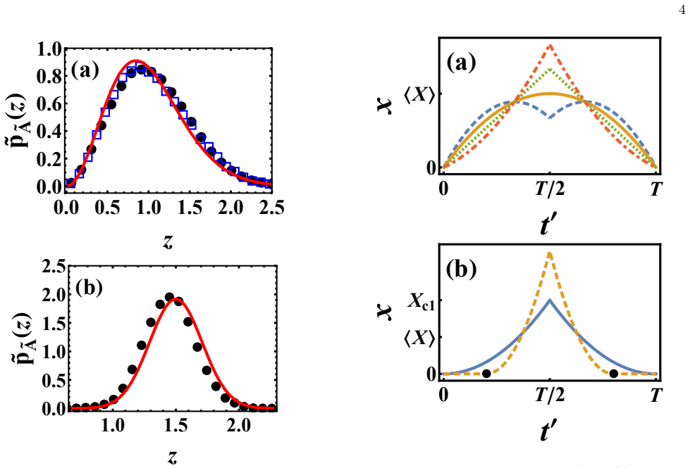
Summary. The paper reports the first experimental measurement of the Airy distribution (AD) using a dilute colloidal suspension, comparing the measured histogram of areas under Vervaat-transformed Brownian excursions with the exact scaling function in Eq. (3). The authors combine the Donsker-Varadhan (DV) formalism and the optimal fluctuation method (OFM) to derive, respectively, the small- and large-area tails of the AD and the single-time position distribution of a Brownian excursion conditioned on a specified area. For small areas they find that this conditional distribution coincides with the Ferrari-Spohn distribution and provide an exact mapping to a parabolic absorbing wall; for large areas they derive Gaussian fluctuations in the subcritical regime and non-Gaussian forms beyond critical values Xc1(t) and Xc2(t), which they interpret as two third-order dynamical phase transitions that merge into a single transition at t=T/2. An appendix derives the tails of the distribution of the area under the square of a Brownian excursion. I checked the algebraic concern raised about Eq. (D5): when the first term is read as a fraction rather than as a product, Eq. (D5) is the correct solution of the area-constraint cubic, and at X=Xc2 (namely ã=2/3) it gives τ/t=2, so the intermediate-regime trajectory satisfies the area constraint; the apparent inconsistency is therefore not present.
Significance. If the results hold, this is a significant paper: it provides the first direct laboratory verification of the Airy distribution, places the known asymptotic tails in a physically transparent large-deviation framework, explains the Ferrari--Spohn coincidence through an exact canonical/microcanonical mapping, and makes falsifiable predictions about third-order dynamical phase transitions in the conditional position distribution. The derivations in Appendices B and D are first-principles and reproduce known tails without adjustable parameters, and the experimental comparison in Fig. 1 is parameter-free. The algebraic error that initially appeared to undermine the second phase transition does not survive scrutiny; what remains are local presentation issues, most notably a cross-reference typo in Appendix D and a need for clearer typesetting of Eq. (D5).
minor comments (6)
- [Appendix D, just below Eq. (D7)] The sentence 'where τ is given by (D6)' should read 'where τ is given by (D5)'; Eq. (D6) is the supercritical trajectory and does not define τ.
- [Appendix D, Eq. (D5)] The first term of Eq. (D5) is line-broken in the present text and is easy to misread as a product. Please typeset it unambiguously as the fraction (2ã−1)^2 / [2(√((2ã−1)^3+1)+1)^{2/3}], or equivalently present τ/t in the explicitly symmetric Cardano form ã+1/2 + (1/2)[(√((2ã−1)^3+1)+1)^{2/3} + (√((2ã−1)^3+1)−1)^{2/3}], so that the area constraint at X=Xc2 is visibly satisfied.
- [Main text, after Eqs. (14)--(16)] The claim that the second critical line Xc2(t) is a third-order transition is stated without an explicit check that the first two derivatives of the large-deviation function are continuous and the third derivative jumps there; adding a one-line verification would make the central claim easier to audit.
- [Abstract and Sec. II] The abstract says there are two singularities for large areas, whereas for the symmetric observation time t=T/2 the two transitions merge into one; please add a qualifier such as 'for generic observation times' to avoid ambiguity.
- [Fig. 2(a)] The experimental conditional averages are based on only 22 (large-area) and 200 (small-area) trajectories; adding error bars or confidence bands would make the agreement with Eqs. (8) and the constant-area prediction quantitative.
- [Fig. 1] The broadening of the measured histogram near the maximum is attributed to particle polydispersity; a quantitative estimate, for example a convolution over a distribution of diffusivities, would strengthen this explanation.
Circularity Check
No significant circularity: the theoretical predictions are derived from independent variational and eigenvalue calculations, then validated against data and simulations rather than fitted.
full rationale
I find no circularity in this paper. The Airy-distribution measurement is a direct histogram of Vervaat-transformed colloidal trajectories compared with the externally known Darling–Louchard/Takács expression (3); no parameter is fitted to the histogram. The small-area tail and the Ferrari–Spohn coincidence are derived from the Donsker–Varadhan tilted-generator eigenvalue problem (Appendix B) and from an exact Laplace-transform/canonical-ensemble mapping (Appendix C), respectively; the Ferrari–Spohn result of Ref. [44] is an external result that is reproduced, not assumed. The large-area rate functions and the two critical lines are obtained by minimizing the Wiener action (7) under the area and position constraints (Appendix D), and the critical values Xc1 and Xc2 are algebraic consequences of the optimal-trajectory formulas, not imported from the authors' prior work. Citations such as Refs. [34]–[37] are used for context and for the delta-function OFM treatment, but they are not load-bearing inputs to the central claims. The paper does not rename a known result: the conditional position distribution p_A(X,t) and its large-deviation branches are new statistics derived from first principles and tested against unconditioned simulations. I note, for the correctness pass rather than the circularity pass, that the printed intermediate-branch formula (D5) appears algebraically inconsistent with the area constraint at Xc2: integrating Eq. (D4) gives tau/t = 2 at a-tilde = 2/3, whereas Eq. (D5) gives tau/t about 2.054. That is an internal mathematical issue in the supporting calculation, not a circular reduction, so it does not change the circularity score.
Assumptions & free parameters
assumptions (7)
- domain assumption Wiener action s[x(t)] = (1/2)∫ ẋ² dt gives the path weight exp(-s/D0) for Brownian trajectories, up to pre-exponential factors.
- domain assumption The Donsker-Varadhan large deviation principle applies to the area of Brownian excursions, so the rate function I(a) is given by the Legendre-Fenchel transform of the SCGF from the ground state energy of the tilted operator.
- domain assumption The optimal fluctuation method gives the large-A tail as the minimizer of the Wiener action subject to the area constraint, with exponentially subleading contributions from other trajectories.
- domain assumption The biased (canonical) ensemble with weight e^{-µA} and the conditioned (microcanonical) ensemble are equivalent in the large-T limit through a Laplace transform and a single saddle point at µ*=µ*(A).
- standard math The tangent construction from one-sided variations yields the correct optimal trajectory when the unconstrained extremum would cross the absorbing boundary at zero.
- standard math The Vervaat transform maps a Brownian bridge into a Brownian excursion, used to build excursions from free trajectories.
- standard math The closed-form series (3) for the Airy distribution f(ξ), obtained from the Laplace transform of Darling and Louchard, is correct.
Cite this review
Pith. "Pith review of The Airy distribution: experiment, large deviations and additional statistics." pith.science (2026). https://pith.science/paper/HCXTCSWU
@misc{pith2026190808354,
  author       = {Pith},
  title        = {Pith review of: The Airy distribution: experiment, large deviations and additional statistics},
  year         = {2026},
  howpublished = {\url{https://pith.science/paper/HCXTCSWU}},
  note         = {Machine review of arXiv:1908.08354}
}
read the original abstract
The Airy distribution (AD) describes the probability distribution of the area under a Brownian excursion. The AD is prominent in several areas of physics, mathematics and computer science. Here we use a dilute colloidal system to directly measure, for the first time, the AD in experiment. We also show how two different techniques of theory of large deviations - the Donsker-Varadhan formalism and the optimal fluctuation method - manifest themselves in the AD. We advance the theory of the AD by calculating, at large and small areas, the position distribution of a Brownian excursion conditioned on a given area, and measure its mean in the experiment. For large areas, we uncover two singularities in the large deviation function, which can be interpreted as dynamical phase transitions of third order. For small areas the position distribution coincides with the Ferrari-Spohn distribution, and we identify the reason for this coincidence.
Figures


Figures from the paper (3 more)


Reference graph
Works this paper leans on
-
[1]
The Airy distribution: experiment, large deviations and additional statistics
= x(t = T ) = 0, and to stay positive, x(t) > 0 for 0<t<T . The area under the Brownian excursion, A = ∫ T 0 x(t)dt, (1) is a random variable characterized by the probability dis- tribution P (A,T ): the AD. The only dimensional pa- rameters entering the problem are A, T and the particle diffusivityD0 [18], and dimensional analysis yields P (A,T ) = 1√D0T ...
work page Pith review arXiv 1908
-
[2]
Large- B tail of P (B,T ) The constrained Lagrangian of the OFM is now L [x(t), ˙x(t)] = ˙x2/2−λx2. The optimal trajectory is x(t) = √ 2B T sin (πt T ) , (E14) where we set λ = π2/(2T 2) to obey the constraint B = ∫T 0 x2(t)dt. Calculating the action from Eq. (7), we finally obtain − lnP (B≫D0T 2)≃ π2B 2D0T 2, (E15) in agreement with Ref. [23]. 11
-
[3]
Note thatN (µ) is the Laplace transform ofP (A), and it is known exactly [7, 8]. Equations (C11)-(C15) provide an exact connection between the conditional probability distributionp (X|A) and the distributionPC (∆X) in the Ferrari-Spohn model with a parabolic wall. 8 In the limit of T→∞ at fixed values of A/T and X (note that this limit implies a small area...
-
[4]
(B5) for ˆH (k)≡ ˆH (−λ), we obtain ˜I(k) =− √ −9k 2 , (E11) where k < 0
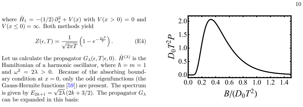
Small- B tail of P (B,T ) By virtue of Eq. (B5) for ˆH (k)≡ ˆH (−λ), we obtain ˜I(k) =− √ −9k 2 , (E11) where k < 0. The Legendre-Fenchel transform (B1) yields the DV rate function I(b) = 9 8b (E12) where b≡B/T . This leads to − lnP (B≪D0T 2)≃ 9D0T 2 8B , (E13) in agreement with Ref. [23]
-
[5]
S. N. Majumdar, Curr. Sci. 89, 2076 (2005)
work page 2005
- [6]
- [7]
- [8]
Show all 69 references
-
[9]
Perrin, Comp
J. Perrin, Comp. Rend. 146, 967 (1908)
1908
-
[10]
Tak´ acs, Adv
L. Tak´ acs, Adv. Appl. Prob. 23, 557 (1991); J. Appl. Prob. 32, 375 (1995)
1991
-
[11]
R. M. Mazo, Brownian Motion: Fluctuations, Dynamics, and Applications (Oxford Science Publications, Oxford, UK, 2008)
2008
-
[12]
D. A. Darling, Ann. Probab. 11, 803 (1983)
1983
-
[13]
Louchard, J
G. Louchard, J. Appl. Probab. 21, 479 (1984)
1984
-
[14]
Tak´ acs, J
L. Tak´ acs, J. Appl. Math. Stoch. Anal.4, 1 (1991)
1991
-
[15]
M. A. Stapleton and K. Christensen J. Phys. A: Math. Gen. 39, 9107 (2006)
2006
-
[16]
Flajolet, P
P. Flajolet, P. Poblete and A. Viola, Algorithmica 22, 490 (1998)
1998
-
[17]
S. N. Majumdar and A. Comtet, Phys. Rev. Lett. 92, 225501 (2004)
2004
-
[18]
S. N. Majumdar and A. Comtet, J. Stat. Phys. 119, 314 (2005)
2005
-
[19]
Schehr and S
G. Schehr and S. N. Majumdar, Phys. Rev. E. 73, 056103 (2006)
2006
-
[20]
Vall´ ee and M
O. Vall´ ee and M. Soares,Airy Functions and Applications to Physics (Imperial College, London, 2004)
2004
-
[21]
Medalion, E
S. Medalion, E. Aghion, H. Meirovitch, E. Barkai and D. A. Kessler, Sci. Rep. 6, 27661 (2016)
2016
-
[22]
Barkai, E
E. Barkai, E. Aghion, and D. A. Kessler, Phys. Rev. X. 4, 021036 (2014)
2014
-
[23]
The Brownian motion can be formally defined by the equation ˙x =√D0ξ(t), where ξ(t) is a delta-correlated zero-mean Gaussian noise,⟨ξ (t)ξ (t′)⟩ =δ (t−t′)
-
[24]
Wolfram Research, Inc., http://functions.wolfram.com/HypergeometricFunctions/
-
[25]
J. C. Crocker and D. G. Grier, J. Colloid Interface Sci 179, 298310 (1996)
1996
-
[26]
Janson, Probab
S. Janson, Probab. Surveys 4, 80 (2007)
2007
-
[27]
M. J. Kearney, S. N. Majumdar and R. J. Martin, J. Phys. A: Math. Theor. 40, 863 (2007)
2007
-
[28]
Cs¨ org¨ o, Z
M. Cs¨ org¨ o, Z. Shi and M. Yor, Bernoulli5, 1035 (1999)
1999
-
[29]
Flajolet and G
P. Flajolet and G. Louchard, Algorithmica 31, 361 (2001)
2001
-
[30]
Colaiori, A
F. Colaiori, A. Baldassarri and C. Castellano, Phys. Rev. E. 69, 041105 (2004)
2004
-
[31]
M. D. Donsker and S. R. S. Varadhan, Comm. Pure Appl. Math. 28, 1 (1975); 28, 279 (1975); 29, 389 (1976); 36, 183 (1983)
1975
-
[32]
Gartner, Th
J. Gartner, Th. Prob. Appl. 22, 24 (1977); R. S. Ellis, Ann. Prob. 12, 1 (1984)
1977
-
[33]
Touchette, Phys
H. Touchette, Phys. Rep. 478, 1 (2009)
2009
-
[34]
Touchette, Physica A 504, 5 (2018)
H. Touchette, Physica A 504, 5 (2018)
2018
-
[35]
N. R. Smith and B. Meerson, J. Stat. Mech. 023205 (2019)
2019
-
[36]
Grosberg and H
A. Grosberg and H. Frisch, J. Phys. A: Math. Gen. 36, 8955 (2003)
2003
-
[37]
In Memoriam Marc Yor - S´ eminaire de Probabilit´ es XLVII
N. Ikeda and H. Matsumoto in “In Memoriam Marc Yor - S´ eminaire de Probabilit´ es XLVII”, edited by C. Donati- Martin, A. Lejay and A. Rouault, Lecture Notes in Math- ematics (Springer, Cham, 2015), vol. 2137, p. 497
2015
-
[38]
Basnayake, A
K. Basnayake, A. Hubl, Z. Schuss and D. Holcman, Phys. Lett. A 382, 3449 (2018)
2018
-
[39]
Meerson, J
B. Meerson, J. Stat. Mech. (2019) 013210
2019
-
[40]
An alternative method, proposed for a generalized Brownian bridge [51, 52, 64], could not be extended to excursions, as it is restricted to Gaussian processes
Methods like Doob’s h-transform [62] are hard to use due to the conditioning on both X and A [54, 63]. An alternative method, proposed for a generalized Brownian bridge [51, 52, 64], could not be extended to excursions, as it is restricted to Gaussian processes
-
[41]
Meerson and N
B. Meerson and N. R. Smith, J. Phys. A: Math. Theor. 52, 415001 (2019)
2019
-
[42]
Meerson, Int
B. Meerson, Int. J. Mod. Phys. B 33, 1950172 (2019)
2019
-
[43]
J. A. Fill and S. Janson, Ann. Comb. 12, 403 (2009)
2009
-
[44]
This unexpected coincidence can be ex- plained by an exact mapping that we found between the two systems
coincide. This unexpected coincidence can be ex- plained by an exact mapping that we found between the two systems. The details of calculation are presented in Appendix C. The mapping involves a biased ensem- ble [45]: an ensemble of excursions, where the proba- bility of each...
-
[45]
Janson and G
S. Janson and G. Louchard, Electron. J. Prob. 12, 1600 (2007)
2007
-
[46]
Chetrite and H
R. Chetrite and H. Touchette, Ann. Henri Poincar´ e 16, 2005 (2015)
2015
-
[47]
Groeneboom, Probab
P. Groeneboom, Probab. Theory Relat. Fields 81, 79 (1989)
1989
-
[48]
Frachebourg and P
L. Frachebourg and P. Martin, J. Fluid Mech. 417, 323 (2000)
2000
-
[49]
P. L. Ferrari and H. Spohn, Ann. Probab. 33, 1302 (2005)
2005
-
[50]
Chetrite and H
R. Chetrite and H. Touchette, Phys. Rev. Lett. 111, 120601 (2013)
2013
-
[51]
D. loffe, S. Shlosman and Y. Velenik, Commun. Math. Phys. 336, 905 (2015)
2015
-
[52]
D. loffe, Y. Velenik and V. Wachtel, Probab. Theory Re- lat. Fields 170, 11 (2018)
2018
-
[53]
loffe and Y
D. loffe and Y. Velenik, Markov Process. Relat. Fields 24, 487 (2018)
2018
-
[54]
Nechaev, K
S. Nechaev, K. Polovnikov, S. Shlosman, A. Valov and A. Vladimirov, Phys. Rev. E 99, 012110 (2019)
2019
-
[55]
Elsgolts, Differential Equations and the Calculus of Variations (Mir Publishers, Moscow, 1977), p
L. Elsgolts, Differential Equations and the Calculus of Variations (Mir Publishers, Moscow, 1977), p. 360
1977
-
[56]
Mazzolo, J
A. Mazzolo, J. Stat. Mech. (2017) P023203
2017
-
[57]
Mazzolo, J
A. Mazzolo, J. Math. Phys. 58, 093302 (2017)
2017
-
[58]
Bertini, A
L. Bertini, A. De Sole, D. Gabrielli, G. Jona-Lasinio and C. Landim, Rev. Mod. Phys. 87, 593 (2015)
2015
-
[59]
N Majumdar and H
S. N Majumdar and H. Orland, J. Stat. Mech. (2015) P06039
2015
-
[60]
Feller, An Introduction to Probability Theory and its Applications (New York, Wiley, 1968)
W. Feller, An Introduction to Probability Theory and its Applications (New York, Wiley, 1968)
1968
-
[61]
Vervaat, Ann
W. Vervaat, Ann. Probab., 7, 143 (1979)
1979
-
[62]
Nguyen The, Combin
M. Nguyen The, Combin. Probab. Comput. 13, 697 (2004)
2004
-
[63]
Redner, A Guide to First-Passage Processes (Cam- bridge University Press, Cambridge, England, 2001)
S. Redner, A Guide to First-Passage Processes (Cam- bridge University Press, Cambridge, England, 2001)
2001
-
[64]
L. D. Landau and E. M. Lifshits, Quantum Mechanics, Non-Relativistic theory (Pergamon, London, 1958)
1958
-
[65]
Wolfram Research, Inc., http://mathworld.wolfram.com/HermitePolynomial.html
-
[66]
Abate and P
J. Abate and P. P. Valk´ o, Int. J. Numer. Meth. Engng. 60, 979 (2004)
2004
-
[67]
J. L. Doob, Classical Potential Theory and its Probabilis- tic Counterpart (Springer, New York, 1984)
1984
-
[68]
S. N. Majumdar and C. Dasgupta, Phys. Rev. E. 73, 011602 (2006)
2006
-
[69]
Sottinen and A
T. Sottinen and A. Yazigi, Stoch. Process. Appl. 124, 3084 (2014)
2014
Reviewed August 14, 2026 · model on record in the stance chip above.
Discussion (0). Continue with ORCID to comment.