REVIEW 4 major objections 6 minor 26 references
A Staged Deep Learning Approach to Spatial Refinement in 3D Temporal Atmospheric Transport
T0 review · 4 major / 6 minor · reviewed 2026-08-11 · deepseek-v4-flash
Pith's one-line read A two-stage neural network predicts 3D plume dispersion roughly 1,000 times faster than LES while beating a high-resolution baseline in accuracy.
desk verdict A solid two-stage surrogate for 3D plume dispersion with a genuine accuracy gain, but the headline speedup and deployment claims hinge on an untested assumption about low-resolution inputs. read the letter →
The pith
A machine-rendered reading of the paper's core claim, the machinery that carries it, and where it could break.
The reading
What carries the argument
The load-bearing mechanism is the staged decomposition into a temporal module (TM) and a spatial refinement module (SRM). The TM is a 3D U-Net with a ConvLSTM bottleneck that ingests a sliding window of five consecutive 10-minute, 8×32×32 concentration fields and emits the next frame; during inference its predictions are fed back recursively. The SRM is a separate 3D U-Net that maps each 8×32×32 predicted field to 32×128×128, producing the advertised fourfold spatial refinement. The argument is that predicting on the coarse grid first keeps the temporal model from trying to resolve fine eddies, and the SRM then adds spatial detail only where the temporal structure is already coherent, which is why errors grow more slowly than in the high-resolution baseline.
What would settle it
Take a genuinely coarse Aeolus simulation (or a sparse array of point sensors) and feed its raw low-resolution concentration fields to DST3D-UNet-SR without downsampling the high-resolution truth; if the four metrics degrade substantially compared with the reported test-set values, the synthetic-input assumption fails. A weaker check is to run the model on wind directions and speeds outside the training ranges (340–360 degrees, 1.5–10 m/s) and see whether the stage separation still contains error growth.
Extended reading notes
Core claim
The central claim is that separating temporal prediction from spatial refinement lets a neural network match or beat a comparable high-resolution temporal model while costing three orders of magnitude less than LES. Working only from low-resolution inputs, the temporal module autoregressively predicts plume concentration fields, and the spatial module then applies a fourfold super-resolution step; on ten held-out LES runs the complete model achieves MSE 1.2 ± 0.4, IoU 0.62 ± 0.08, SSIM 0.84 ± 0.03, and mass-conservation error 0.3 ± 0.3, outperforming the high-resolution baseline on the averaged metrics. The authors also show that feeding new observational data into the temporal module during inference improves predictions near the source and lets the model track a late-time concentration plateau. In their telling, the dual-stage structure keeps errors from compounding because fine spatial detail is added only after the coarse temporal evolution is established.
Load-bearing premise
The load-bearing premise is that low-resolution inputs created by downsampling high-resolution LES output are faithful stand-ins for the coarse data the model would receive in real operation, so that training on synthetic coarse fields does not hide a mismatch with true low-resolution physics.
Editorial extensions
If this is right
- If the performance on downsampled LES transfers to operational inputs, a 5-hour plume forecast becomes available in seconds per time step rather than the roughly 2.25 hours of LES, opening the door to real-time emergency response.
- Because the staged modules are trained independently, either the temporal predictor or the spatial upsampler can be upgraded without retraining the other.
- The model's ability to ingest new observations during inference means operational forecasts can be nudged as sensor data arrive, improving accuracy where concentrations are highest.
- The comparison metrics indicate the staged model beats a high-resolution temporal baseline with comparable parameter count on MSE, SSIM, and mass conservation, and ties on IoU.
- The 4x spatial refinement sits well within the range where volumetric super-resolution has been shown to work, so the same dual-stage recipe is a plausible template for other 3D transport problems.
Reading between the lines
- A natural next test the authors do not run is to train or fine-tune on true coarse-resolution simulations rather than downsampled high-resolution fields; if that works, the acceleration claim extends to settings where only coarse models or sparse sensor networks are available.
- The staged design is not specific to xenon plumes; it could be transferred to any advection-diffusion system in complex geometry where temporal dynamics are smooth on a coarse grid but fine spatial structure matters.
- The headline 1,000x speedup is computed against the full LES runtime, not against another neural baseline; the practical gain is therefore largest when simulations are repeated many times, since the training cost is amortized over those runs.
Signed reviews
Editorial analysis
A structured set of objections, weighed in public.
Referee Report
Summary. The paper proposes DST3D-UNet-SR, a two-stage deep learning model for three-dimensional plume dispersion. A temporal module (TM) predicts plume evolution on low-resolution 8×32×32 grids from five-frame windows, and a spatial refinement module (SRM) upsamples the outputs by 4× to 32×128×128. The model is trained on 80 high-resolution Aeolus LES runs, validated on 10, and tested on 10 runs with varying wind speed and direction. The authors compare against a high-resolution temporal baseline (HRTM) with similar parameter count and report MSE, IoU, SSIM, and conservation of mass over 33 time steps, together with inference timings. They claim a three-orders-of-magnitude speedup over LES and a sensor-point validation using synthetic sensor locations in the Aeolus fields. The central empirical result is that DST3D-UNet-SR achieves competitive or better metrics than HRTM while using low-resolution input and faster inference.
Significance. If the performance and speedup claims hold, the staged architecture is a useful contribution to real-time plume forecasting, especially for emergency response and uncertainty quantification. The modular design is well motivated, and the comparison against HRTM, a same-cost baseline operating directly on high-resolution data, is a fairer test than a pure upsampling baseline. The paper reports means and standard deviations over 10 test runs rather than single cherry-picked examples, and the figures show qualitative error fields. The main limitations are the untested synthetic low-resolution input assumption and the ambiguous end-to-end speedup accounting; these do not invalidate the core architecture but must be resolved before the deployment claims can be accepted.
major comments (4)
- [III, IV-B, VII] The paper never fixes a single definition of the low-resolution inputs. Section III says the LR data are created from HR LES fields using skimage.transform.resize, whereas Section IV-B says the SRM training inputs are generated by average pooling the high-resolution ground truth. These are different operations, and the reported test metrics do not state which one was used. More fundamentally, both operations produce noise-free deterministic projections of the same HR field that serves as the target, allowing the model to exploit the specific coarsening kernel. The load-bearing assumption that such inputs are representative of operational LR fields, for example from a coarse LES or a sensor-assimilation system, is untested. The sensor validation in Section VII does not close this gap because it resamples the same Aeolus LES and explicitly uses no field data. The authors should either evaluate on natively coarse LES runs or clearly restrict the claims to the downsampled-data regime.
- [VI] The speedup comparison is not end-to-end. The 0.35 s per time step is the cost of a single low-resolution-input to high-resolution-output prediction on a cropped 5 km × 5 km × 2 km domain, while the 2.25 h "original simulation runtime" is the total runtime of the full-domain LES. To claim a three-orders-of-magnitude speedup, the authors need to compare the total forecast wall-clock time, including LR input generation, the autoregressive rollout of the 33 frames, and any required initial coarse simulation, against the LES runtime for the same forecast horizon and domain. As written, the factor mixes a per-step inference cost with a total simulation cost, so the headline acceleration claim is not established.
- [VIII and Table I] The statement that DST3D-UNet-SR outperforms HRTM across all key metrics is stronger than the data support. Table I shows identical IoU (0.62 vs 0.62) and overlapping MSE values (1.2 ± 0.4 vs 1.5 ± 0.4), so without a paired significance test only SSIM and CM clearly favor DST3D-UNet-SR. The conclusion and abstract should be qualified to avoid overstating the accuracy advantage.
- [VII and Figure 10] The "dynamic adaptation" demonstration uses ground-truth sensor values from the same Aeolus simulation as additional inputs at 1 h, 1.5 h, and 2.5 h. This shows that the model can exploit perfect additional information, but it does not demonstrate robustness to realistic observational noise, sparse or irregular sampling, or sensor error. The abstract's claim that the model "demonstrates the ability to dynamically adapt to evolving conditions through the incorporation of new observational data" should be softened to reflect the simulation-based and noise-free nature of these updates.
minor comments (6)
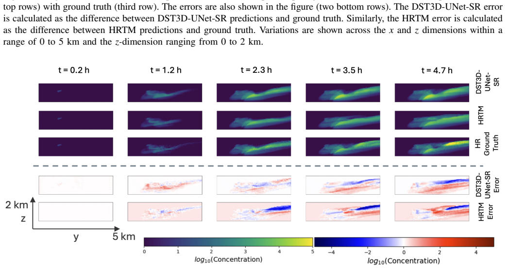
- [V and Figure 4] The text in Section V says Figure 4 shows variations across the y- and z-plane, but the figure caption says the x-z plane; please reconcile the axes and ranges.
- [Abstract] The abstract contains "DST3DUNet-SR" without the hyphen; use "DST3D-UNet-SR" consistently.
- [Appendix A1] The description of enc3 lists "BatchNorm3d(2)" after a Conv3d layer with 7×64 channels; this appears to be a typo, likely BatchNorm3d(64) or similar.
- [VI] The inference timings (0.35 ± 0.01 s and 1.58 ± 0.01 s) are reported without specifying the hardware, batch size, or whether data transfer and preprocessing are included; please add these details for reproducibility.
- [VI] The IoU threshold of log10(Concentration) = 1 is introduced without a sensitivity analysis; a short justification or a sensitivity check would make the metric more robust.
- [III] The text says the simulation spans five hours but later states that 330 one-minute steps were retained as 33 ten-minute steps, which is 5.5 hours; please make the time spans consistent.
Circularity Check
No significant circularity: the neural surrogate is trained on held-out LES runs, evaluated against an independent HRTM baseline, and its claims do not reduce by construction to its inputs.
full rationale
The paper's central claim is that a two-stage deep learning model (TM followed by SRM) can emulate LES plume dispersion faster and with competitive accuracy. This is a surrogate-modeling claim, not a first-principles derivation, so the usual circularity patterns do not apply. The model is trained on 80 LES runs and evaluated on 10 held-out test runs, and the reported metrics in Table I compare DST3D-UNet-SR against a separately trained HRTM baseline with comparable parameter count. No fitted parameter is renamed as a prediction: the TM predicts low-resolution next frames in an autoregressive loop and the SRM upsamples those frames, with both modules optimized against MSE on the same LES ground truth. Self-citations appear in the related-work and design-justification context (for example, prior CNN, LSTM, and super-resolution studies by the authors), but none of these citations carries the central accuracy or speedup claim, nor do they import a uniqueness theorem or forbid alternative architectures. The Section VII sensor validation is admittedly not an independent field-data test, because it compares against sensor locations sampled from the same Aeolus simulation used for training, and the paper explicitly states that direct comparison with experiments is not possible; this is a limitation in external validity, not circularity. There is a minor internal inconsistency in how low-resolution inputs are generated (skimage resize in Section III versus average pooling in Section IV-B), and the synthetic low-resolution inputs are deterministic coarsenings of the same LES fields, which raises a deployment-generalization concern, but that is a correctness/robustness issue rather than a derivation that reduces to its own inputs. Under the hard-rule standard requiring a quotable equation or fit that is equivalent to the claimed result, I find no circular step.
Assumptions & free parameters
free parameters (5)
- temporal window size =
5 time steps
- IoU threshold =
log10(Concentration) = 1
- training duration =
33 time steps at 10-minute intervals
- downsampling method =
skimage.transform.resize (Section III) vs average pooling (Section IV-B)
- domain crop =
[2, 5, 5] km
assumptions (4)
- domain assumption Low-resolution data generated by downsampling high-resolution LES is representative of true low-resolution atmospheric fields
- domain assumption Aeolus LES output is accurate ground truth for plume dispersion
- domain assumption The wind speed and direction ranges sampled by Latin Hypercube Sampling cover the intended operating envelope
- standard math Standard deep learning training assumptions (MSE loss, Adam optimizer, train/validation/test split on independent runs)
Cite this review
Pith. "Pith review of A Staged Deep Learning Approach to Spatial Refinement in 3D Temporal Atmospheric Transport." pith.science (2026). https://pith.science/paper/HGH365LA
@misc{pith2026241210945,
  author       = {Pith},
  title        = {Pith review of: A Staged Deep Learning Approach to Spatial Refinement in 3D Temporal Atmospheric Transport},
  year         = {2026},
  howpublished = {\url{https://pith.science/paper/HGH365LA}},
  note         = {Machine review of arXiv:2412.10945}
}
read the original abstract
High-resolution spatiotemporal simulations effectively capture the complexities of atmospheric plume dispersion in complex terrain. However, their high computational cost makes them impractical for applications requiring rapid responses or iterative processes, such as optimization, uncertainty quantification, or inverse modeling. To address this challenge, this work introduces the Dual-Stage Temporal Three-dimensional UNet Super-resolution (DST3D-UNet-SR) model, a highly efficient deep learning model for plume dispersion prediction. DST3D-UNet-SR is composed of two sequential modules: the temporal module (TM), which predicts the transient evolution of a plume in complex terrain from low-resolution temporal data, and the spatial refinement module (SRM), which subsequently enhances the spatial resolution of the TM predictions. We train DST3DUNet- SR using a comprehensive dataset derived from high-resolution large eddy simulations (LES) of plume transport. We propose the DST3D-UNet-SR model to significantly accelerate LES simulations of three-dimensional plume dispersion by three orders of magnitude. Additionally, the model demonstrates the ability to dynamically adapt to evolving conditions through the incorporation of new observational data, substantially improving prediction accuracy in high-concentration regions near the source. Keywords: Atmospheric sciences, Geosciences, Plume transport,3D temporal sequences, Artificial intelligence, CNN, LSTM, Autoencoder, Autoregressive model, U-Net, Super-resolution, Spatial Refinement.
Figures


Figures from the paper (6 more)



Reference graph
Works this paper leans on
-
[1]
G. Camps-Valls, D. Tuia, X. X. Zhu, and M. Reichstein, Deep learning for the Earth Sciences: A comprehensive approach to remote sensing, climate science and geosciences . John Wiley & Sons, 2021. ARTIFICIAL INTELLIGENCE IN GEOSCIENCES, VOL. X, NO. X, NOVEMBER XXXX 11
work page 2021
-
[2]
Predicting wind- driven spatial deposition through simulated color images using deep autoencoders,
M. G. Fern ´andez-Godino, D. D. Lucas, and Q. Kong, “Predicting wind- driven spatial deposition through simulated color images using deep autoencoders,” Scientific Reports, vol. 13, no. 1, p. 1394, 2023
work page 2023
-
[3]
Deep convolutional autoencoders as generic feature extractors in seismological applications,
Q. Kong, A. Chiang, A. C. Aguiar, M. G. Fern ´andez-Godino, S. C. Myers, and D. D. Lucas, “Deep convolutional autoencoders as generic feature extractors in seismological applications,” Artificial intelligence in geosciences, vol. 2, pp. 96–106, 2021
work page 2021
-
[4]
Image super-resolution using deep convolutional networks,
C. Dong, C. C. Loy, K. He, and X. Tang, “Image super-resolution using deep convolutional networks,” IEEE Transactions on Pattern Analysis and Machine Intelligence , vol. 38, no. 2, pp. 295–307, 2015
work page 2015
-
[5]
W. T. Chung, B. Akoush, P. Sharma, A. Tamkin, K. S. Jung, J. H. Chen, J. Guo, D. Brouzet, M. Talei, B. Savard, A. Y . Poludnenko, and M. Ihme, “Turbulence in Focus: Benchmarking Scaling Behavior of 3D V olumetric Super-Resolution with BLASTNet 2.0 Data,” Advances in Neural Information Processing Systems (NeurIPS) , vol. 36, 2023
work page 2023
-
[6]
A. Marcos Filho, M. C. Santos, and C. M. Pereira, “Exploring lstm- based prediction for radioactive plume atmospheric dispersion in nuclear power plant emergencies: A preliminary study,” Nuclear Engineering and Design, vol. 419, p. 112982, 2024
work page 2024
-
[7]
Accelerating high-strain continuum- scale brittle fracture simulations with machine learning,
M. G. Fern ´andez-Godino, N. Panda, D. O’Malley, K. Larkin, A. Hunter, R. T. Haftka, and G. Srinivasan, “Accelerating high-strain continuum- scale brittle fracture simulations with machine learning,” Computational Materials Science, vol. 186, p. 109959, 2021
work page 2021
-
[8]
Uncertainty bounds for multivariate machine learning predic- tions on high-strain brittle fracture,
C. Garcia-Cardona, M. G. Fern ´andez-Godino, D. O’Malley, and T. Bhat- tacharya, “Uncertainty bounds for multivariate machine learning predic- tions on high-strain brittle fracture,” Computational Materials Science , vol. 201, p. 110883, 2022
work page 2022
Show all 26 references
-
[9]
Stressnet-deep learning to predict stress with fracture propagation in brittle materials,
Y . Wang, D. Oyen, W. Guo, A. Mehta, C. B. Scott, N. Panda, M. G. Fern´andez-Godino, G. Srinivasan, and X. Yue, “Stressnet-deep learning to predict stress with fracture propagation in brittle materials,” Npj Materials Degradation, vol. 5, no. 1, p. 6, 2021
2021
-
[10]
Spatiotemporal predictions of toxic urban plumes using deep learning,
Y . Wang, M. G. Fern ´andez-Godino, N. Gunawardena, D. D. Lucas, and X. Yue, “Spatiotemporal predictions of toxic urban plumes using deep learning,” arXiv preprint arXiv:2406.02582 , 2024
2024 arXiv
-
[11]
A hybrid spatiotem- poral deep model based on cnn and lstm for air pollution prediction,
S. Tsokov, M. Lazarova, and A. Aleksieva-Petrova, “A hybrid spatiotem- poral deep model based on cnn and lstm for air pollution prediction,” Sustainability, vol. 14, no. 9, p. 5104, 2022
2022
-
[12]
Capturing plume behavior in complex terrain: an overview of the Nevada National Security Site Meteorological Experiment (METEX21),
S. Wharton, M. J. Brown, D. Dexheimer, J. D. Fast, R. K. Newsom, W. W. Schalk, and D. J. Wiersema, “Capturing plume behavior in complex terrain: an overview of the Nevada National Security Site Meteorological Experiment (METEX21),” Frontiers in Earth Science , vol. 11, p. 1251...
2023
-
[13]
Real-time xenon sensor analysis report PNNL- 35939,
S. Stave, K. Bertschinger, S. Emmons, E. Becker, J. Fast, E. Siciliano, and M. Zalavadia, “Real-time xenon sensor analysis report PNNL- 35939,” Pacific Northwest National Laboratory, Tech. Rep., 2024
2024
-
[14]
Large Eddy Simulations of Turbulent and Buoyant Flows in Urban and Complex Terrain Areas Using the Aeolus Model,
A. A. Gowardhan, D. L. McGuffin, D. D. Lucas, S. J. Neuscamman, O. Alvarez, and L. G. Glascoe, “Large Eddy Simulations of Turbulent and Buoyant Flows in Urban and Complex Terrain Areas Using the Aeolus Model,” Atmosphere, vol. 12, no. 9, p. 1107, sep 2021
2021
-
[15]
Large sample properties of simulations using Latin hypercube sampling,
M. Stein, “Large sample properties of simulations using Latin hypercube sampling,” Technometrics, vol. 29, no. 2, pp. 143–151, 1987
1987
-
[16]
On the use of symmetries in building surrogate models,
M. Giselle Fern ´andez-Godino, S. Balachandar, and R. T. Haftka, “On the use of symmetries in building surrogate models,” Journal of Mechanical Design, vol. 141, no. 6, p. 061402, 2019
2019
-
[17]
Adam: A method for stochastic optimization,
D. P. Kingma and J. Ba, “Adam: A method for stochastic optimization,” arXiv preprint arXiv:1412.6980 , 2014
2014 arXiv
-
[18]
Goodfellow, Y
I. Goodfellow, Y . Bengio, and A. Courville, Deep learning. MIT press, 2016
2016
-
[19]
The distribution of the flora in the alpine zone. 1,
P. Jaccard, “The distribution of the flora in the alpine zone. 1,” New Phytologist, vol. 11, no. 2, pp. 37–50, 1912
1912
-
[20]
Image quality assessment: from error visibility to structural similarity,
Z. Wang, A. C. Bovik, H. R. Sheikh, and E. P. Simoncelli, “Image quality assessment: from error visibility to structural similarity,” IEEE Transactions on Image Processing , vol. 13, no. 4, pp. 600–612, 2004
2004
-
[21]
R. J. LeVeque, Finite volume methods for hyperbolic problems . Cam- bridge university press, 2002, vol. 31. APPENDIX A. DualStage Temporal 3D UNet-SR Model Architecture The DualStage Temporal 3D UNet-SR architecture is de- signed to enhance the temporal resolution and spatial ...
2002
-
[22]
Its architecture comprises 3,214,401 trainable parameters
Temporal Module: The TM is constructed using a con- volutional autoencoder architecture, incorporating ConvLSTM layers at its bottleneck to capture temporal dependencies within the input data. Its architecture comprises 3,214,401 trainable parameters. It operates on input data...
-
[23]
• dec2: ConvTranspose3d(7 × 32, 7 × 16, 2, stride =
followed by BatchNorm3d, ReLU activation, and Dropout3d(0.2). • dec2: ConvTranspose3d(7 × 32, 7 × 16, 2, stride =
-
[24]
• dec3: ConvTranspose3d(7×16, 1, 2, stride = 2)followed by ReLU activation
followed by BatchNorm3d, ReLU activation, and Dropout3d(0.2). • dec3: ConvTranspose3d(7×16, 1, 2, stride = 2)followed by ReLU activation. The TM generates single time-step predictions with an output shape of (batch size , 1, 8, 32, 32), which are recursively fed back into the ...
-
[25]
Its architecture has 951,873 trainable parameters
Spatial Refinement Module: The SRM processes the TM output, reshaping it to (batch size , 8, 32, 32) and produces high-resolution output of shape (batch size, 32, 128, 128). Its architecture has 951,873 trainable parameters. Encoder: • enc1: Conv3d(1, 7 × 16, 3, padding = 1) f...
-
[26]
followed by ReLU activation. Like the TM, the HRTM produces single time-step pre- dictions with an output shape of (batch size, 1, 32, 128, 128), which are recursively fed back into the model in a sliding window framework consisting of five time steps
Reviewed August 11, 2026 · model on record in the stance chip above.
Discussion (0). Continue with ORCID to comment.