REVIEW 3 major objections 4 minor 23 references
PI-GINOT: Data-free geometry-informed neural operator learning for finite-strain hyperelasticity on parametric DogBone specimens
T0 review · 3 major / 4 minor · reviewed 2026-07-31 · deepseek-v4-flash
Pith's one-line read A physics-constrained neural operator predicts how a four-parameter family of DogBone specimens stretches and carries load, trained without finite-element data by enforcing equilibrium, traction, and load transfer directly.
desk verdict A carefully scoped proof of concept that a geometry-conditioned operator can be trained without FEM labels for finite-strain hyperelasticity; the validation numbers are plausible but currently sit on an unverified custom Abaqus UEL. read the letter →
The pith
A machine-rendered reading of the paper's core claim, the machinery that carries it, and where it could break.
The reading
What carries the argument
The carrying mechanism is the separation of geometry encoding from physics decoding: a boundary point cloud is encoded by a hierarchical point-set network into latent geometry tokens, and a cross-attention transformer decoder conditions a query-point displacement prediction on those tokens. Two supporting pieces do the heavy lifting: the hard boundary-condition layer, which constructs the displacement field as u = ūξ + ξ(1−ξ)ϕu, v = ηϕv so the essential constraints hold for any network output, and the internal axial section-force consistency loss, which integrates the axial first Piola–Kirchhoff stress over vertical sections and penalizes variation of the resultant along the specimen—a globa
What would settle it
Take the most demanding validation geometry (the narrow-gauge FE08) and run a systematic mesh-refinement study or a comparison against a built-in plane-stress hyperelastic element in the same commercial solver; if the reference displacement or peak-stress values shift by more than the claimed error margins, the central claim is not a true measure of PI-GINOT.
Extended reading notes
Core claim
PI-GINOT maps a DogBone specimen's boundary point cloud to its finite-strain hyperelastic displacement field under a fixed 1 mm grip displacement. A geometry encoder turns the point cloud into latent tokens; a cross-attention decoder predicts displacement at arbitrary query points, with essential boundary conditions enforced exactly through a constructed admissible layer instead of soft penalties. Stresses are not learned: automatic differentiation plus a compressible Neo-Hookean plane-stress closure (a local differentiable Newton solve) produces them. The training objective is purely physical—equilibrium, traction-free boundaries, symmetry tractions, a determinant barrier, and an internal s
Load-bearing premise
The reported 2.1–7.1% displacement and stress accuracy numbers measure against a custom finite-element reference that the paper does not show to be mesh-converged or independently verified, so the reference's accuracy is the load-bearing premise for every headline number.
Editorial extensions
If this is right
- Finite-strain response families can be explored without regenerating finite-element data: once trained, the operator answers new DogBone geometries at arbitrary query points in a single forward pass.
- Exact displacement-boundary enforcement plus a purely physical loss keeps predictions kinematically admissible; the paper attributes remaining error to local stress-gradient resolution, not boundary-condition drift.
- The accuracy hierarchy (displacements best, peak von Mises moderate, component-wise stresses worst) makes the method usable for geometry screening and load-transfer estimates but not for fatigue- or fracture-level local stress assessment.
- Internal section-force consistency serves as a global equilibrium diagnostic: the four strongest validation cases keep mean section-force errors between 1.7% and 3.7%, with the narrow-gauge case worst at 10.2%.
- Stress errors concentrated at the gauge-fillet transition identify a concrete target—local derivative resolution—for future architecture changes such as curvature-biased sampling or multi-scale features.
Reading between the lines
- Because the failure mode is localized to the gauge-fillet transition, curvature-biased or adaptive collocation near the fillet is a testable fix: if component-wise stress errors shrink faster than displacement errors, the gradient-resolution story is confirmed.
- The same architecture and loss could extend to multi-load or multi-material inputs; the open question is whether the section-force term still keeps global equilibrium consistent when the displacement mode is no longer a single linear ramp.
- Practically, the accuracy mix (good displacements and peaks, weak stress components) suggests a hybrid workflow: neural screening of geometry families with finite-element refinement reserved for flagged hot spots—an engineering use the authors imply but do not claim.
- The latent-swap and boundary-resampling diagnostics indicate the geometry tokens genuinely carry shape information; a follow-up could separate encoder error from decoder error by feeding analytic boundary features directly.
Signed reviews
Editorial analysis
A structured set of objections, weighed in public.
Referee Report
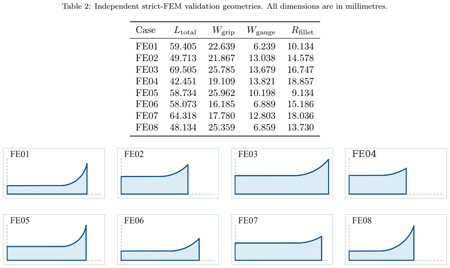
Summary. This paper introduces PI-GINOT, a physics-informed geometry-informed neural operator transformer for finite-strain hyperelastic plane-stress problems on a four-parameter family of DogBone specimens. The geometry is encoded from a boundary point cloud into latent tokens; a cross-attention decoder predicts displacements at arbitrary points. Essential boundary conditions are hard-enforced, stresses are obtained by automatic differentiation with a compressible Neo-Hookean plane-stress closure, and training uses equilibrium, traction, symmetry, determinant-barrier and section-force consistency losses without any FEM displacement/stress labels. Abaqus/Standard with a custom UEL is used only for post-training validation. On eight held-out geometries the model reports displacement L2 errors of 2.1%–7.1%, signed peak von Mises errors of 0.9%–13.3%, component stress errors of 10.0%–47.6% and section-force errors not exceeding 10.3%. The paper is explicit about the stress-gradient limitation near the gauge-fillet transition and about the controlled scope of the study.
Significance. If the central claim is established, this is a noteworthy contribution: it would be the first demonstration of a data-free geometry-conditioned neural operator for finite-strain hyperelasticity on a parametric shape family, with a clean separation between physics-based training and FEM validation. Strengths include the hard boundary-condition layer, the section-force consistency diagnostic, validation on eight independent geometries spanning the parameter range, and an honestly stratified error reporting that distinguishes displacement, peak von Mises, component stress and section-force accuracy. The method is reproducible in principle, but the supplied details are incomplete — final loss weights are missing and the custom FE reference is not yet shown to be trustworthy. The contribution is best read as a proof of concept rather than a production surrogate.
major comments (3)
- [Section 7; Tables 3–4] The validation reference is a custom Abaqus/Standard user element, described only as "implemented specifically for this study", with no mesh-refinement study, no analytical patch test, and no comparison against a built-in model. Every headline error — displacement 2.1–7.1%, peak von Mises 0.9–13.3%, section-force ≤10.3% — is measured relative to this reference. The small CV_FE values in Table 4 show internal consistency of the FE solution but not correctness or mesh convergence. Please add: (a) a patch test of the UEL, (b) a mesh-convergence study on at least one smooth case and one narrow-gauge case (e.g., FE04 and FE08), and (c) a cross-check against Abaqus's built-in hyperelastic plane-stress formulation or an analytical solution. Without this, the reported accuracy is a difference between two approximations and the central validation claim is unverified.
- [Section 6.2, Table 1, Eq. (31)] The exact final loss configuration is not fully reported. Table 1 gives w_eq = 150, w_trac = 4–60, and w_N = 80, but omits w_part and w_bar from Eq. (31). The thresholds J_min (Eq. (28)) and epsilon_N (Eq. (30)) are not stated. The text also says "additional emphasis" is placed on curved traction-free boundaries and section-force consistency without specifying the values. Since the weighted physics objective defines the method and the final model, these omissions preclude exact reproduction. Please report exact final weights and thresholds, or provide a precise selection procedure.
- [Section 6.2; Tables 3–4] All reported errors are from a single training run; no seed variation or repeated runs are given. Collocation resampling and Adam initialization are stochastic, so it is unclear whether the stated ranges — e.g., 2.1–7.1% displacement error — are stable. Add mean ± std over at least three seeds for the main metrics, or explicitly state that a single seed is used and discuss sensitivity. This is important for any claim about "the final PI-GINOT model" as a reusable operator.
minor comments (4)
- [Section 9.7] The paper acknowledges that no complete ablation study is included. This is acceptable for a first proof of concept, but the contribution list in Section 1 presents the composite objective as a contribution. A minimal ablation dropping L_bar and L_N would help attribute the observed improvement and strengthen the contribution claims.
- [Section 2.3, Eq. (7)] The displacement \bar{u} appears as an operator input in Eq. (7), but the text states it is fixed to 1 mm and not used as an additional network input. Please clarify that Eq. (7) is the mathematical operator form and that \bar{u} is not an active input dimension.
- [Appendix A] The diagnostics discussion mentions late-stage fluctuations after approximately 1450 epochs. Please report the total number of training epochs and the stopping criterion used for the final model.
- [Data and code availability] The code "will be made available in a public repository upon publication." Given the custom UEL used for validation, please include the UEL source or a complete element formulation (residual and consistent tangent) in the supplementary material so that reviewers and readers can verify the reference solutions.
Circularity Check
No significant circularity: PI-GINOT is trained purely on physics residuals and validated only post-training against independent Abaqus references.
full rationale
The derivation chain is not circular. The central claim is that a geometry-conditioned operator can be trained without finite-element displacement or stress labels and then validated against finite-element solutions. The training loss (Section 5) consists of interior equilibrium residuals (Eq. 25), traction-free and symmetry traction residuals (Eqs. 26-27), a determinant barrier (Eq. 28), and an internal section-force consistency term (Eqs. 29-30). None of these terms uses Abaqus output: the section-force term penalizes variation of the axial resultant N(s), which is computed from the predicted P11 field and is a physical consequence of equilibrium, not a fitted FEM target. Essential boundary conditions are imposed exactly by the hard layer (Eq. 23) rather than learned from data. The paper repeatedly states that Abaqus references are used only after training: 'Abaqus simulations are used only after training for validation' and 'The finite-element data are not used in training, loss weighting or model fitting.' Thus the reported errors are genuine post-training comparisons against independent finite-element solutions. The one substantive concern—that the custom UEL reference is not accompanied by a mesh-refinement or patch-test study—is a question of reference-solution trustworthiness, not circularity: it does not make the prediction equivalent to its inputs by construction. There are also no load-bearing self-citations or imported uniqueness theorems; the GINOT-related citations are prior-architecture context, not used to define the present physics objective or to force its conclusions. Accordingly, no circular step can be exhibited, and the appropriate score is 0.
Assumptions & free parameters
free parameters (3)
- Loss weights w_eq, w_trac, w_N (and unreported w_part, w_bar) =
150; 4–60; 80; not reported
- J_min and epsilon_N in determinant barrier and section-force loss =
not reported
- Collocation/architecture hyperparameters (Nb=320, Ntok=32, d=64, 6000/2400 points) =
as listed in Table 1
assumptions (4)
- domain assumption Quarter-domain symmetry reduction (Section 2.1-2.2): the upper-right quarter with u(0,Y)=0, u(Lhalf,Y)=ū, v(X,0)=0 represents the full DogBone.
- domain assumption Plane-stress closure P33(F2D,F33)=0 has a unique physical root at every point and the Newton solve is accurate through autodiff (Section 3.2).
- ad hoc to paper The custom Abaqus UEL used as validation ground truth is a correct and converged implementation (Section 7).
- domain assumption Internal axial section force N(s) should be nearly constant, so penalizing its coefficient of variation is a valid physics constraint (Eqs. 29-30).
Cite this review
Pith. "Pith review of PI-GINOT: Data-free geometry-informed neural operator learning for finite-strain hyperelasticity on parametric DogBone specimens." pith.science (2026). https://pith.science/paper/HJ7IHWWM
@misc{pith2026260723299,
  author       = {Pith},
  title        = {Pith review of: PI-GINOT: Data-free geometry-informed neural operator learning for finite-strain hyperelasticity on parametric DogBone specimens},
  year         = {2026},
  howpublished = {\url{https://pith.science/paper/HJ7IHWWM}},
  note         = {Machine review of arXiv:2607.23299}
}
read the original abstract
Parametric nonlinear solid-mechanics simulations are widely used in virtual testing, optimisation, and uncertainty analysis, but repeated finite-element simulations become costly when geometry changes. This paper presents PI-GINOT, a physics-informed neural operator that predicts finite-strain hyperelastic responses across a four-parameter family of DogBone specimens without using finite-element training data. Each specimen is described by a boundary point cloud, which is encoded into geometry features. A cross-attention decoder then predicts displacement at arbitrary points. Displacement boundary conditions are enforced exactly, while stresses are computed using automatic differentiation and a compressible Neo-Hookean plane-stress model. Training is guided by equilibrium, traction-free and symmetry conditions, deformation stability, and internal force consistency. Abaqus simulations are used only after training for validation. Across eight test geometries, PI-GINOT achieves displacement errors of 2.1%-7.1%, peak von Mises stress errors of 0.9%-13.3%, and section-force errors below 10.3%. Larger errors occur in individual stress components, especially for narrow specimens, mainly because of steep stress gradients near the gauge-to-fillet transition. These results show that PI-GINOT can provide useful geometry-dependent predictions for nonlinear solid mechanics without labelled simulation data, while also revealing where better local stress resolution is still needed.
Figures


Figures from the paper (6 more)



Reference graph
Works this paper leans on
-
[1]
D. W. Abueidda, Q. Lu, S. Koric, Meshless physics-informed deep learning method for three-dimensional solid mechanics, International Journal for Numerical Methods in Engineering 122 (2021) 7182–7201
2021
-
[2]
Bonet, R
J. Bonet, R. D. Wood, Nonlinear Continuum Mechanics for Finite Element Analysis, second ed., Cambridge University Press, Cambridge, 2008
2008
-
[3]
E. Haghighat, M. Raissi, A. Moure, H. Gomez, R. Juanes, A deep learning framework for solution and discovery in solid mechanics, arXiv:2003.02751, 2020
arXiv 2003
-
[4]
Haghighat, R
E. Haghighat, R. Juanes, SciANN: A Keras/TensorFlow wrapper for scientific computations and physics- informed deep learning using artificial neural networks, Computer Methods in Applied Mechanics and Engineering 373 (2021) 113552
2021
-
[5]
G. A. Holzapfel, Nonlinear Solid Mechanics: A Continuum Approach for Engineering, Wiley, Chichester, 2000
2000
-
[6]
G. E. Karniadakis, I. G. Kevrekidis, L. Lu, P. Perdikaris, S. Wang, L. Yang, Physics-informed machine learning, Nature Reviews Physics 3 (2021) 422–440
2021
-
[7]
Kovachki, Z
N. Kovachki, Z. Li, B. Liu, K. Azizzadenesheli, K. Bhattacharya, A. Stuart, A. Anandkumar, Neural operator: Learning maps between function spaces with applications to PDEs, Journal of Machine Learning Research 24 (2023) 1–97
2023
-
[8]
Z. Li, N. Kovachki, K. Azizzadenesheli, B. Liu, K. Bhattacharya, A. Stuart, A. Anandkumar, Neural operator: Graph kernel network for partial differential equations, arXiv:2003.03485, 2020
arXiv 2003
Show all 23 references
-
[9]
Z. Li, N. Kovachki, K. Azizzadenesheli, B. Liu, K. Bhattacharya, A. Stuart, A. Anandkumar, Multipole graph neural operator for parametric partial differential equations, in: Advances in Neural Information Processing Systems, 2020
2020
-
[10]
Z. Li, N. Kovachki, K. Azizzadenesheli, B. Liu, K. Bhattacharya, A. Stuart, A. Anandkumar, Fourier neural operator for parametric partial differential equations, in: International Conference on Learning Representations, 2021
2021
-
[11]
Q. Liu, W. Zhong, H. Meidani, D. Abueidda, S. Koric, P. Geubelle, Geometry-informed neural operator transformer for partial differential equations on arbitrary geometries, Computer Methods in Applied Mechanics and Engineering 451 (2026) 118668. 28
2026
-
[12]
L. Lu, P. Jin, G. Pang, Z. Zhang, G. E. Karniadakis, Learning nonlinear operators via DeepONet based on the universal approximation theorem of operators, Nature Machine Intelligence 3 (2021) 218–229
2021
-
[13]
Mildenhall, P
B. Mildenhall, P. P. Srinivasan, M. Tancik, J. T. Barron, R. Ramamoorthi, R. Ng, NeRF: Representing scenes as neural radiance fields for view synthesis, in: European Conference on Computer Vision, 2020, pp. 405–421
2020
-
[14]
V. M. Nguyen-Thanh, X. Zhuang, T. Rabczuk, A deep energy method for finite deformation hyperelas- ticity, European Journal of Mechanics – A/Solids 80 (2020) 103874
2020
-
[15]
C. R. Qi, L. Yi, H. Su, L. J. Guibas, PointNet++: Deep hierarchical feature learning on point sets in a metric space, in: Advances in Neural Information Processing Systems, 2017
2017
-
[16]
Raissi, P
M. Raissi, P. Perdikaris, G. E. Karniadakis, Physics-informed neural networks: A deep learning framework for solving forward and inverse problems involving nonlinear partial differential equations, Journal of Computational Physics 378 (2019) 686–707
2019
-
[17]
C. Rao, H. Sun, Y. Liu, Physics-informed deep learning for computational elastodynamics without labeled data, Journal of Engineering Mechanics 147 (2021) 04021043
2021
-
[18]
Samaniego, C
E. Samaniego, C. Anitescu, S. Goswami, V. M. Nguyen-Thanh, H. Guo, K. Hamdia, X. Zhuang, T. Rabczuk, An energy approach to the solution of partial differential equations in computational mechanics via machine learning: Concepts, implementation and applications, Computer Method...
2020
-
[19]
J. C. Simo, T. J. R. Hughes, Computational Inelasticity, Springer, New York, 1998
1998
-
[20]
Sukumar, A
N. Sukumar, A. Srivastava, Exact imposition of boundary conditions with distance functions in physics- informed deep neural networks, Computer Methods in Applied Mechanics and Engineering 389 (2022) 114333
2022
-
[21]
Vaswani, N
A. Vaswani, N. Shazeer, N. Parmar, J. Uszkoreit, L. Jones, A. N. Gomez, L. Kaiser, I. Polosukhin, Attention is all you need, in: Advances in Neural Information Processing Systems, 2017
2017
-
[22]
C. Zeng, Y. Zhang, J. Zhou, Y. Wang, Z. Wang, Y. Liu, L. Wu, D. Z. Huang, Point cloud neural operator for parametric PDEs on complex and variable geometries, Computer Methods in Applied Mechanics and Engineering 443 (2025) 118022
2025
-
[23]
Zhong, H
W. Zhong, H. Meidani, Physics-Informed Geometry-Aware Neural Operator, Computer Methods in Applied Mechanics and Engineering 434 (2025) 117540. 29
2025
Reviewed July 31, 2026 · model on record in the stance chip above.
Discussion (0). Continue with ORCID to comment.