REVIEW 3 major objections 4 minor 66 references
The Influence of the Memory Capacity of Neural DDEs on the Universal Approximation Property
T0 review · 3 major / 4 minor · reviewed 2026-08-15 · deepseek-v4-flash
Pith's one-line read The paper claims that the expressivity of neural delay differential equations is controlled by the memory capacity Kτ — the product of the vector field's Lipschitz constant and the delay — so that universal approximation fails for small…
desk verdict A solid threshold result for globally defined neural DDEs, but the abstract sells a cleaner and more general picture than the theorems actually deliver. read the letter →
The pith
A machine-rendered reading of the paper's core claim, the machinery that carries it, and where it could break.
The reading
What carries the argument
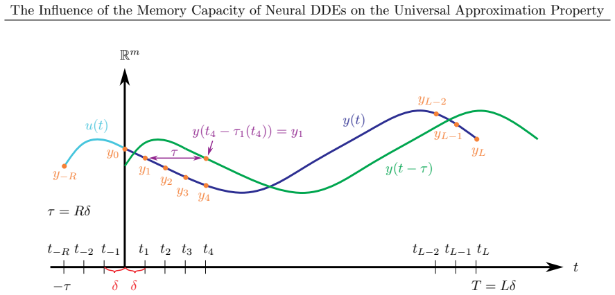
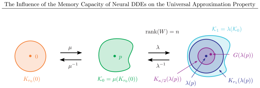
The load-bearing object is the memory capacity Kτ: the delay τ is the length of the longest shortcut connection in the DenseResNet whose infinite-depth limit is the neural DDE, and K is the global Lipschitz constant of the vector field, the continuous analogue of how strongly the activation functions amplify differences between layers. The negative side rests on the small-delay theory of functional differential equations. When Kτe < 1, every solution of the DDE is exponentially attracted to a finite-dimensional inertial manifold whose points are 'special solutions', and those special solutions are exactly the solutions of a single ordinary differential equation, so the infinite-dimensional system behaves like an ODE with only a mild Lipschitz inflation. The positive side rests on a direct construction: the vector field is built so that on [0, τ] the delayed argument equals the constant input, the target value Ψ(x) is reached by explicit integration at time τ, and the field then switches off, yielding exact embedding for every globally Lipschitz Ψ. The negative proof enforces the obstruction by choosing a Morse function — smooth with non-degenerate critical points — as the target and using the Jordan–Brouwer separation theorem to show that the output map's level sets cannot separate the interior from the boundary of a ball around the extremum.
What would settle it
Decisive test: try to approximate the scalar target x ↦ x² to accuracy ε < r₀²/2 on a ball using any non-augmented neural DDE with Kτe < 1 whose vector field is defined only on a proper open subset of the history space; success would show the small-memory obstruction does not cover the most general architecture, while failure would confirm that the obstruction is tied to the memory threshold itself.
Extended reading notes
Core claim
The paper's central claim is that the universal approximation property of neural DDEs is governed by the memory capacity Kτ — the product of the global Lipschitz constant K of the vector field and the delay τ — not by the mere fact that the phase space is infinite-dimensional. For globally defined, weakly nonlinear vector fields with Kτe < 1, no non-augmented neural DDE with bounded weights can approximate certain smooth targets: the paper constructs a smooth function with a non-degenerate local extreme point and proves, via exponential attraction toward ODE-governed special solutions and a level-set separation argument, that every such network misses it by a fixed positive error (Theorems 5.4 and 3.13). For Kτ ≥ 2(1 + KΨ/(w w̃)), in contrast, any globally Lipschitz continuous map can be embedded exactly as the time-T map of a non-augmented neural DDE with Lipschitz constant K and delay τ — the universal embedding property (Theorem 3.9) — and with dimension m ≥ n + q the embedding works for every delay, including zero (Theorem 3.14). Read together, the theorems map out a transition: increasing Kτ carries the architecture from ODE-like failure, through an uncharacterized intermediate window, to exact representation of all Lipschitz targets.
Load-bearing premise
The negative results assume the vector field is defined on the whole space of continuous histories, globally Lipschitz, and bounded at zero, and the paper does not prove that vector fields living only on proper open subsets can be extended with the same Lipschitz constant and bound.
Editorial extensions
If this is right
- Non-augmented neural DDEs and their parameterized versions inherit the expressivity limits of non-augmented neural ODEs whenever Kτ is below roughly 1/e: no amount of weight tuning or parameterization choice can give them the universal approximation property (Theorems 3.13 and 3.4(a)).
- Once Kτ ≥ 2(1 + KΨ/(w w̃)), any globally Lipschitz target is exactly representable, so the memory threshold functions as a design prescription: to enlarge what a DenseResNet-style architecture can express, increase the longest shortcut length or the amplification of the vector field.
- For augmented architectures with m ≥ n + q, universal embedding holds even at τ = 0, so memory is not what unlocks expressivity when the state dimension already exceeds input plus output; the benefit of Kτ is specific to the non-augmented case.
- The obstruction is generic rather than pathological: Morse functions with local extrema are dense in the spaces of smooth functions, so the failing target is not a specially crafted exception.
Reading between the lines
- The paper's parameter regions leave an uncharacterized window between Kτe < 1 (no approximation) and Kτ ≥ 2 (universal embedding); a natural conjecture, not tested here, is that the true critical curve lies inside this window and is set by the spectral gap of the linearized small-delay operator rather than by the two explicit thresholds.
- Transferred back through the Euler discretization of Section 2.1, the threshold predicts a critical shortcut length for discrete DenseResNets: networks whose longest inter-layer connection spans fewer than roughly 1/(Kδ) layers should exhibit the same approximation obstructions as plain ResNets — a quantitative architectural prediction that could be tested numerically without training full continu
- Because the positive construction writes the target Ψ directly into the vector field, its practical counterpart is a parameterized family rich enough to approximate every weakly nonlinear field on [0, T] × C; Theorem 3.4(b) makes universality for concrete parameterized architectures conditional on exactly that richness, so checking it becomes the real engineering question.
- The level-set separation mechanism suggests the obstruction is topological: local extrema force an interior-versus-boundary separation that Lipschitz-small DDE flows cannot achieve, whereas saddle points are explicitly expected to be approximable — implying that classification-type output functions with well-separated level sets may sit right at the boundary of what small-memory networks can learn
Signed reviews
Editorial analysis
A structured set of objections, weighed in public.
Referee Report
Summary. The paper studies universal approximation and universal embedding for neural delay differential equations (neural DDEs), interpreted as infinite-depth limits of DenseResNets, and investigates how the product Kτ of the vector-field Lipschitz constant and the delay controls expressivity. The main positive result (Theorem 3.9) is an explicit construction embedding any globally Lipschitz map into a non-augmented neural DDE when Kτ is sufficiently large, with a similar augmented construction (Theorem 3.14) when the DDE dimension is at least n+q. The main negative result (Theorem 3.13, Corollary 5.5, Theorem 5.4) states that when Kτ is sufficiently small, non-augmented neural DDEs cannot have the universal approximation property, using the exponential attraction of DDE solutions to finite-dimensional special solutions and a topological separation argument involving local extreme points. The paper concludes that the infinite-dimensional phase space alone does not give universal approximation and that a memory threshold Kτ is needed.
Significance. If the claims held in the stated generality, this would be a valuable contribution: the positive construction in Theorem 3.9 is explicit, and the negative proof in Section 5 carefully tracks constants while combining small-delay theory, exponential attraction, Morse theory, and Jordan-Brouwer separation. The paper also connects the continuous-time results to DenseResNet architectures through the Euler-discretization discussion in Section 2. However, both sides of the claimed phase transition require attention before the advertised conclusion is justified: the positive construction has an unverified domain-of-definition issue, and the negative theorems are proved only for vector fields that are globally defined on all of C, not for the general architecture of Definition 2.7.
major comments (3)
- [Section 5.5, Step 3; Theorem 4.14] The no-go theorem is proved only for vector fields F: Ω_t×C→R^m that are globally defined in the second variable. Theorem 4.14, which is invoked in Step 3 of the proof of Theorem 5.4, extends exactly this class: it assumes Ω_y=C and does not apply to the general architecture of Definition 2.7, where F may be defined only on an open Ω=Ω_t×Ω_y. Consequently, Corollary 5.5 and Theorem 3.13 inherit the global-domain restriction, while the abstract and Theorem 3.13 present the result for non-augmented neural DDEs without this restriction. A separate argument, or a Lipschitz/C^{0,k}_b extension theorem for local vector fields that preserves K and A, is needed; without it the small-capacity no-go claim overstates what is proved.
- [Section 3.3; Figure 3.2] The Lipschitz constant K in the positive and negative regimes is not the same object. In Theorem 3.9 the constructed vector field is only shown to be Lipschitz on R×Ω_0, the set of constant initial data, and the proof's estimate is performed for y_t,z_t∈Ω_0; no Lipschitz bound on all of C or on Ω_y is established. In Theorem 3.13 and Theorem 5.4, K is a global Lipschitz constant on Ω_t×C. Thus the regions AUE and AnUA in Figure 3.2 are defined under different hypotheses, and the claimed Kτ-transition is not a phase diagram for one fixed function class. The comparison requires either strengthening the positive theorem to a globally Lipschitz vector field on all of C or relaxing the negative theorem's assumption.
- [Section 3.3, proof of Theorem 3.9] The proof does not show that the solution segments of the constructed DDE remain in the domain Ω_y, so the vector field may not be well-defined on the whole interval [0,T]. The solution y(t) interpolates between λ(x) and (1/\tilde w)Id_{m,q}Ψ(x); for a general open, nonconvex X, the first n components of y(t) need not remain in wX for t∈(0,τ], so y_t may leave Ω_y before the vector field becomes zero on (τ,∞). The proof asserts unique solvability without verifying y_t∈Ω_y. This affects the central positive embedding claim. A fix is to enlarge the domain (for example, require the condition only at the delayed evaluation point u(-τ) for t∈[0,τ] and define F=0 on all of C for t≥τ, or extend Ψ to all of R^n with the same Lipschitz constant).
minor comments (4)
- [Corollary 5.5; Theorem 5.4] Corollary 5.5 states τ∈[0,τ0(K)], while Theorem 5.4 is proved only for τ∈[0,τ0(K)); the proof's final contradiction uses strict inequalities, so either the closed interval should be justified or the statement should use τ<τ0(K).
- [Theorems 3.9 and 3.13] The notation NDDE^k_{τ,N,K} is used before the subscript K is formally defined in the class notation; please state explicitly that K denotes the Lipschitz constant and specify on which domain it is measured in each theorem.
- [Definition 3.8] Calling the property 'globally Lipschitz continuous on Ω_t×Ω_0' is potentially confusing when Ω_0 is a subset; consider using 'Lipschitz continuous on Ω_t×Ω_0' to avoid suggesting global Lipschitz continuity on all of C.
- [Lemma 5.15] In the definition of τ3, the condition r_0^2-2ε-δ*>0 is guaranteed by the assumptions but should be stated explicitly before dividing by ln(2C_2/(r_0^2-2ε-δ*)).
Circularity Check
No significant circularity: main results are derived from explicit constructions and external DDE/Morse/Jordan-Brouwer theorems; self-citations are background only.
full rationale
The derivation chain is self-contained for its central claims. The positive universal embedding theorems (3.9 and 3.14) are proven by explicitly writing down the vector field F and integrating it exactly on the relevant time interval; the Lipschitz constant K is then estimated from that same constructed vector field, and the threshold Kτ ≥ 2(1+KΨ/(w w̃)) is an inequality on the constructed K, not an assumed equality. The negative results (Theorem 5.4, Corollary 5.5, Theorem 3.13) rest on Driver's special-solution existence, Jarnik-Kurzweil exponential attraction, Hale-Lunel DDE well-posedness, the Morse-Palais lemma, and the Jordan-Brouwer separation theorem—all external to the present authors. The proof tracks the error terms δ1,t*, δ2,β, δ3,τ explicitly and derives the no-approximation contradiction from them; nothing is fitted to the target map Ψ or renamed as a prediction. The author self-citations [32,33] are used only as background: [32] for the standard augmented-neural-ODE embedding idea (which Theorem 3.14 reproves by direct construction) and [33] for the generic-density statement about Morse functions, which is not needed for the obstruction since Corollary 5.5 exhibits a concrete quadratic Ψ. A limitation exists: Theorem 5.4 is proved for globally defined weakly nonlinear vector fields F: Ω_t × C → R^m, and Theorem 4.14 extends only such fields; this is a scope restriction, not circularity, because the proof does not assume the conclusion it is trying to establish. No equation is equivalent to its input by construction, and no fitted parameter is relabeled as a prediction.
Assumptions & free parameters
assumptions (6)
- standard math Existence, uniqueness, and continuous dependence of DDE solutions (Hale-Lunel).
- standard math Special solutions exist and attract all solutions exponentially when Kτe < 1 (Driver, Jarnik-Kurzweil).
- standard math Special solutions satisfy an ODE on an inertial manifold with Lipschitz constant |λ1| < Ke (Theorem 4.11).
- standard math Jordan-Brouwer separation theorem and Morse-Palais lemma.
- domain assumption The vector field of the neural DDE is globally defined, weakly nonlinear, with uniform bound ∥F(t,0)∥ ≤ A.
- domain assumption Constant initial data are used for the DDE to maintain the DenseResNet analogy.
Cite this review
Pith. "Pith review of The Influence of the Memory Capacity of Neural DDEs on the Universal Approximation Property." pith.science (2026). https://pith.science/paper/HJUKEZLL
@misc{pith2026250507244,
  author       = {Pith},
  title        = {Pith review of: The Influence of the Memory Capacity of Neural DDEs on the Universal Approximation Property},
  year         = {2026},
  howpublished = {\url{https://pith.science/paper/HJUKEZLL}},
  note         = {Machine review of arXiv:2505.07244}
}
abstract
Neural Ordinary Differential Equations (Neural ODEs), which are the continuous-time analog of Residual Neural Networks (ResNets), have gained significant attention in recent years. Similarly, Neural Delay Differential Equations (Neural DDEs) can be interpreted as an infinite depth limit of Densely Connected Residual Neural Networks (DenseResNets). In contrast to traditional ResNet architectures, DenseResNets are feed-forward networks that allow for shortcut connections across all layers. These additional connections introduce memory in the network architecture, as typical in many modern architectures. In this work, we explore how the memory capacity in neural DDEs influences the universal approximation property. The key parameter for studying the memory capacity is the product $K \tau$ of the Lipschitz constant and the delay of the DDE. In the case of non-augmented architectures, where the network width is not larger than the input and output dimensions, neural ODEs and classical feed-forward neural networks cannot have the universal approximation property. We show that if the memory capacity $K\tau$ is sufficiently small, the dynamics of the neural DDE can be approximated by a neural ODE. Consequently, non-augmented neural DDEs with a small memory capacity also lack the universal approximation property. In contrast, if the memory capacity $K\tau$ is sufficiently large, we can establish the universal approximation property of neural DDEs for continuous functions. If the neural DDE architecture is augmented, we can expand the parameter regions in which universal approximation is possible. Overall, our results show that by increasing the memory capacity $K\tau$, the infinite-dimensional phase space of DDEs with positive delay $\tau>0$ is not sufficient to guarantee a direct jump transition to universal approximation, but only after a certain memory threshold, universal approximation holds.
Figures


Figures from the paper (18 more)





Reference graph
Works this paper leans on
-
[1]
V. Arnold. On the representation of continuous functions of three variables as superpositions of continuous functions of two variables , volume 114, pages 47–133. Springer Berlin Heidelberg,
-
[2]
M. K. Baskar, M. Karafiat, L. Burget, K. Vesely, F. Grezl, and J. Cernocky. Residual memory networks: Feed-forward approach to learn long-term temporal dependencies. pages 4810–4814,
-
[3]
R. T. Q. Chen, Y. Rubanova, J. Bettencourt, and D. Duvenaud. Neural ordinary differential equations. NeurIPS, 2018. doi:10.48550/ARXIV.1806.07366. 56 The Influence of the Memory Capacity of Neural DDEs on the Universal Approximation Property
-
[4]
C. Chicone. Inertial and slow manifolds for delay equations with small delays. Journal of Differential Equations, 190(2):364–406, 2003. doi:10.1016/s0022-0396(02)00148-1
-
[5]
C. Chicone. Inertial flows, slow flows, and combinatorial identities for delay equations. Journal of Dynamics and Differential Equations , 16(3):805–831, 2004. doi:10.1007/s10884-004-6696-4
-
[6]
C. Cipriani, M. Fornasier, and A. Scagliotti. From NeurODEs to AutoencODEs: A mean-field control framework for width-varying neural networks.European Journal of Applied Mathematics, 36(2):188–230, 2024. doi:10.1017/S0956792524000032
-
[7]
R. M. Corless, G. H. Gonnet, D. E. G. Hare, D. J. Jeffrey, and D. E. Knuth. On the LambertW function. Advances in Computational Mathematics , 5(1):329–359, 1996. doi: 10.1007/BF02124750
-
[8]
G. Cybenko. Approximation by superpositions of a sigmoidal function. Mathematics of Control, Signals, and Systems , 2(4):303–314, 1989. doi:10.1007/BF02551274
Show all 66 references
- [9]
-
[10]
R. Diestel. Graph Theory. Springer Berlin Heidelberg, 2025. doi:10.1007/978-3-662-70107-2
2025 doi
-
[11]
R. D. Driver. Existence and stability of solutions of a delay-differential system. Archive for Rational Mechanics and Analysis , 10(1):401–426, 1962. doi:10.1007/BF00281203
1962 doi
-
[12]
R. D. Driver. On ryabov’s asymptotic characteization of the solutions of quasi-linear differential equations with small delays. SIAM Review, 10(3):329–341, 1968. doi:10.1137/1010058
1968 doi
-
[13]
R. D. Driver. Linear differential systems with small delays. Journal of Differential Equations , 21(1):148–166, 1976. doi:10.1016/0022-0396(76)90022-x
1976 doi
- [14]
-
[15]
Glorot and Y
X. Glorot and Y. Bengio. Understanding the difficulty of training deep feedforward neural networks. In International Conference on Artificial Intelligence and Statistics , 2010. URL: https://api.semanticscholar.org/CorpusID:5575601
2010
-
[16]
Guckenheimer and P
J. Guckenheimer and P. Holmes. Nonlinear Oscillations, Dynamical Systems, and Bifurcations of Vector Fields , volume 42 of Applied Mathematical Sciences . Springer New York, 7 edition,
-
[17]
J. K. Hale and S. M. V. Lunel. Introduction to Functional Differential Equations. Springer New York, 1993. doi:10.1007/978-1-4612-4342-7
1993 doi
-
[18]
Hammouamri, I
I. Hammouamri, I. Khalfaoui-Hassani, and T. Masquelier. Learning delays in spiking neural networks using dilated convolutions with learnable spacings. 2023. doi:10.48550/arXiv.2306. 17670
2023 doi
-
[19]
Hanin and M
B. Hanin and M. Sellke. Approximating continuous functions by ReLU nets of minimal width
-
[20]
P. Hartman. Ordinary Differential Equations, volume 38 of Classics in Applied Mathematics. So- ciety for Industrial and Applied Mathematics, 2 edition, 2002. doi:10.1137/1.9780898719222
2002 doi
-
[21]
K. He, X. Zhang, S. Ren, and J. Sun. Deep residual learning for image recognition. IEEE Conference on Computer Vision and Pattern Recognition , pages 770–778, 2016. doi:10.1109/ cvpr.2016.90
2016
-
[22]
M. W. Hirsch. Differential Topology, volume 33 of Graduate Texts in Mathematics . Springer New York, 1976. doi:10.1007/978-1-4684-9449-5 . 57 The Influence of the Memory Capacity of Neural DDEs on the Universal Approximation Property
1976 doi
-
[23]
Hochreiter and J
S. Hochreiter and J. Schmidhuber. Long short-term memory. Neural Computation, 9(8):1735– 1780, 1997. doi:10.1162/neco.1997.9.8.1735
1997 doi
-
[24]
K. Hornik. Approximation capabilities of multilayer feedforward networks. Neural Networks, 4(2):251–257, 1991. doi:10.1016/0893-6080(91)90009-T
1991 doi
-
[25]
Hornik, M
K. Hornik, M. Stinchcombe, and H. White. Multilayer feedforward networks are universal ap- proximators. Neural Networks, 2(5):359–366, 1989. doi:10.1016/0893-6080(89)90020-8
1989 doi
-
[26]
Huang, Z
G. Huang, Z. Liu, L. Van Der Maaten, and K. Q. Weinberger. Densely connected convolutional networks. 2017. doi:10.1109/CVPR.2017.243
2017 doi
-
[27]
Jarnik and J
J. Jarnik and J. Kurzweil. Ryabov’s special solutions of functional differential equations. Boll. Un. Mat. Ital. , (4) 11(3, suppl.):198–208, 1975
1975
- [28]
- [29]
-
[30]
Kolmogorov
A. Kolmogorov. On the representation of continuous functions of several variables as superposi- tions of continuous functions of a smaller number of variables.Dokl. Akad. Nauk, 108(2):179–182, 1956
1956
-
[31]
Kratsios
A. Kratsios. The universal approximation property - characterization, construction, representa- tion, and existence. Annals of Mathematics and Artificial Intelligence , 89(5-6):435–469, 2021. doi:10.1007/s10472-020-09723-1
2021 doi
- [32]
-
[33]
Kuehn and S.-V
C. Kuehn and S.-V. Kuntz. Analysis of the geometric structure of neural networks and neural ODEs via morse functions. Preprint, 2024. doi:10.48550/ARXIV.2405.09351
2024 doi
-
[34]
J. M. Lee. Introduction to Smooth Manifolds , volume 218 of Graduate Texts in Mathematics . Springer New York, 2 edition, 2013. doi:10.1007/978-1-4419-9982-5
2013 doi
-
[35]
E. L. Lima. The jordan-brouwer separation theorem for smooth hypersurfaces. The American Mathematical Monthly, 95(1):39–42, 1988. doi:10.2307/2323445
1988 doi
- [36]
- [37]
- [38]
-
[39]
M. Morse. The Calculus of Variations in the Large , volume 18 of Colloquium Publications . American Mathematical Society, 1934
1934
-
[40]
R. R. Palais. The morse lemma for banach spaces. Bulletin of the American Mathematical Society, 75(5):968–971, 1969
1969
- [41]
-
[42]
A. Pinkus. Approximation theory of the MLP model in neural networks. Acta Numerica, 8:143– 195, 1999. doi:10.1017/s0962492900002919. 58 The Influence of the Memory Capacity of Neural DDEs on the Universal Approximation Property
1999 doi
-
[43]
Ronneberger, P
O. Ronneberger, P. Fischer, and T. Brox. U-Net: Convolutional networks for biomedical image segmentation. pages 234–241, 2015. doi:10.1007/978-3-319-24574-4_28
2015 doi
-
[44]
Ruiz-Balet, E
D. Ruiz-Balet, E. Affili, and E. Zuazua. Interpolation and approximation via momentum ResNets and neural ODEs. Systems & Control Letters , 162:105182, 2022. doi:10.1016/j.sysconle. 2022.105182
2022
-
[45]
Ruiz-Balet and E
D. Ruiz-Balet and E. Zuazua. Neural ODE control for classification, approximation, and trans- port. SIAM Review, 65(3):735–773, 2023. doi:10.1137/21M1411433
2023 doi
-
[46]
Ruthotto and E
L. Ruthotto and E. Haber. Deep neural networks motivated by partial differential equations
- [47]
- [48]
- [49]
-
[50]
A. M. Sch¨ afer and H. G. Zimmermann.Recurrent Neural Networks Are Universal Approximators, pages 632–640. Springer Berlin Heidelberg, 2006. doi:10.1007/11840817_66
2006 doi
- [51]
-
[52]
H. Smith. An Introduction to Delay Differential Equations with Applications to the Life Sciences. Texts in Applied Mathematics. Springer New York, 2011. doi:10.1007/978-1-4419-7646-8
2011 doi
- [53]
-
[54]
W. Wang, X. Li, J. Yang, and T. Lu. Mixed link networks. 2018. doi:10.48550/arXiv.1802. 01808
2018 doi
-
[55]
E. Weinan. A proposal on machine learning via dynamical systems. Commun. Math. Stat, 5:1–11,
-
[56]
Sharkovskii
A. Sharkovskii. Co-existence of cycles of a continuous map of the line into itself. International Journal of Bifurcation and Chaos, 05(05):1263–1273, 1995. English translation: Int. J. Bif. Chaos 5(5), pp. 1263–1273, 1995. doi:10.1142/s0218127495000934
1995 doi
- [57]
- [58]
- [59]
- [60]
-
[61]
doi:10.1007/s40304-017-0103-z
- [62]
-
[2002]
doi:10.1007/978-1-4612-1140-2
-
[2009]
doi:10.1007/978-3-642-01742-1_6
-
[2017]
doi:10.1109/ICASSP.2017.7953070
2017
- [2018]
Reviewed August 15, 2026 · model on record in the stance chip above.
Discussion (0). Continue with ORCID to comment.