Autoregressive Projective Quantum Monte Carlo: From a Hermitian to a Non-Hermitian Perspective

Flore K. Kunst; Lavoisier Wah; Remmy Zen

REVIEW 4 major objections 5 minor 57 references

Autoregressive Projective Quantum Monte Carlo: From a Hermitian to a Non-Hermitian Perspective

T0 review · 4 major / 5 minor · reviewed 2026-08-11 · deepseek-v4-flash

Challenge this review Re-run · record.json Download PDF Read on arXiv ↗ Review JSON

Pith's one-line read Autoregressive PQMC: an RNN guide sharpens ground-state energies to about $10^{-6}$ relative error, for both Hermitian and PT-symmetric non-Hermitian Ising chains.

desk verdict Solid Hermitian RNN-PQMC method, but the non-Hermitian claim is undermined by the real-imaginary decomposition and unreported ξ. read the letter →

arxiv 2608.09496 v1 pith:HOUWECPM submitted 2026-08-10 quant-ph cond-mat.str-el

Lavoisier Wah , Remmy Zen , Flore K. Kunst This is my paper · ORCID

classification quant-phcond-mat.str-el

keywords projectivequantumMonteCarlorecurrentneuralnetworkwavefunctionsautoregressivesamplingself-learningPQMCnon-Hermitiansystemstransverse-fieldIsingchainsignproblemstates

verification ladder T0 review T1 audit T2 compute T3 formal

The pith

A machine-rendered reading of the paper's core claim, the machinery that carries it, and where it could break.

The reading

The paper introduces autoregressive projective quantum Monte Carlo (PQMC), where a recurrent neural network supplies the guiding wavefunction and is retrained on the walker distribution every few projection steps. It claims this guided version is substantially more accurate than standard unguided PQMC while retaining polynomial cost, for both Hermitian and non-Hermitian Hamiltonians. On the staggered transverse-field Ising chain the method reaches relative energy errors around $10^{-5}$ to $10^{-6}$ for systems of 50--150 spins and beats a variational RNN by roughly two orders of magnitude. A sympathetic reader should care because PQMC is a leading method for sign-problem-free Hamiltonians, and a reliable self-learning guide removes its main practical bottleneck: the need for a good hand-built or separately optimized trial state.

What carries the argument

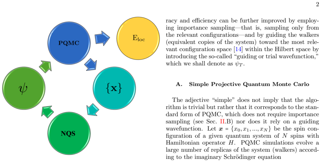
The load-bearing mechanism is the self-learning loop, not any single network design. A recurrent neural network parameterizes the guiding wavefunction through the autoregressive chain rule, so every spin configuration gets an explicit normalized probability and can be sampled exactly, in sequence, without a sampling step over hidden units. Each PQMC stint uses that RNN for importance sampling and continuous-time imaginary-time propagation; the walker configurations are then fed back as training data for a maximum-likelihood (relative-entropy) update of the network parameters. The autoregressive factorization makes this fit cheap and stable, and the continuous-time propagation removes finite-time-step bias. For the non-Hermitian model, a local unitary gauge rotation turns the complex off-diagonal terms into a stoquastic Hamiltonian, and the local energy is evaluated with a biorthogonal mixed estimator that needs only the right ground state.

What would settle it

Run the same self-learning loop on a stoquastic Hamiltonian with a known exact ground state that a one-layer RNN cannot represent exactly, such as a frustrated two-dimensional Ising model, and check whether the mixed-estimator energy converges to the exact value as stints grow; a capacity-dependent plateau would indicate that the loop's fixed point is biased by the ansatz. For the non-Hermitian model, monitor the imaginary part of the local energy after the gauge rotation: persistent nonzero values would signal that the walk is not sampling the true right ground state.

Watch

Extended reading notes

Core claim

The paper's central claim is that a recurrent neural network can act as a self-improving guiding wavefunction inside projective quantum Monte Carlo (PQMC), and that this combination is substantially more accurate than the unguided version at polynomial cost. At each stint, the RNN's autoregressive wavefunction $\psi_{\theta_s}(x)$ is used for importance sampling; the walkers generated by imaginary-time projection are then used to retrain the RNN by maximizing the likelihood of the walker configurations, equivalently minimizing the relative entropy between the network distribution and the walker distribution. The paper shows that after about five stints the mixed-estimator energy stabilises at the exact ground-state energy of the Hermitian staggered transverse-field Ising chain, with relative errors of $2.3\times10^{-6}$, $5.9\times10^{-6}$, and $1.2\times10^{-5}$ at $N=50$, $100$, and $150$ spins, and that the same loop works for a PT-symmetric non-Hermitian Ising chain after a unitary gauge rotation makes the Hamiltonian sign-problem-free. The method outperforms variational RNNs and unguided PQMC in both accuracy and variance.

Load-bearing premise

The method assumes that repeatedly retraining the RNN on the current PQMC walker distribution converges to the true ground state rather than to a biased fixed point, and that five to ten stints are enough; the paper supports this with stint-by-stint energy plots for two models, not with a proof.

Editorial extensions

If this is right

For a Hermitian staggered transverse-field Ising chain with up to 150 spins, the guided method's relative energy error is about two orders of magnitude smaller than a variational RNN's and remains below $10^{-5}$.
The number of stints needed for convergence stays around five to ten across system sizes, about four times fewer than the RBM-guided self-learning PQMC baseline.
The same RNN-guided pipeline applies to PT-symmetric non-Hermitian Ising chains after a gauge rotation, so non-Hermitian ground-state energies can be obtained without a separate variational optimization.
The computational cost remains polynomial in system size, with wall-clock times comparable to unguided PQMC for the system sizes tested.
Because the mixed estimator is not variational, the method's accuracy is tied to the quality of the guide; the more expressive the RNN, the smaller the fluctuations around the true ground state.

Reading between the lines

Editorial extensions of the paper, not claims the author makes directly.

If the self-learning loop converges for the same reason in other stoquastic models, the recipe should transfer to higher-dimensional and frustrated lattices, provided the RNN ansatz can represent the relevant correlations; the paper benchmarks only one-dimensional chains.
The gauge-rotation trick is model-specific; applying the method to a non-Hermitian Hamiltonian without a known stoquastic rotation would test whether the sign-problem mitigation, rather than the RNN guide, is the limiting ingredient.
The biorthogonal mixed estimator uses only the right ground state; the same framework could be extended to left-ground-state observables or to excited states by symmetry projection, which the paper does not explore.

Share X Bluesky LinkedIn Reddit HN

Editorial analysis

A structured set of objections, weighed in public.

Desk editor's note, referee report, and a circularity audit.

Desk Editor's Note

read the letter

The Hermitian half of this paper is a solid contribution; the non-Hermitian half does not support the abstract's 'regardless' claim. The genuinely new piece is using an autoregressive RNN as the guiding wavefunction inside self-learning PQMC. That combination is new, and the Hermitian benchmarks are convincing: the staggered Ising chain has an exact JWB solution, the ED and JWB agree, and the RNN-guided PQMC reaches relative errors around 1e-5 to 1e-6 with lower variance than unguided PQMC. The comparison against variational RNNs is also honest and shows a real improvement on these 1D models. That part is worth taking seriously.

The soft spots are in the non-Hermitian extension. The paper describes a gauge rotation and a real-imaginary decomposition in Appendix C.4. The decomposition is explicitly 'sampling the ground state of the manifestly stoquastic Hermitian Hamiltonian H_eta' and then evaluating ⟨iξD⟩ as a mixed estimator. That means the walkers never feel the iξD term. At the self-learning fixed point the RNN guide is trained to the H_eta ground state, not the H ground state, and by symmetry ⟨D⟩ vanishes on that state. The paper says this is exact when the guide is a good approximation to the ground state of H itself, but the guide is being trained on H_eta walkers, so that condition is circular. If the main NH results in Fig. 9 use the gauge rotation instead, that method is sound in principle, but the paper never states which method produced Fig. 9, and it never reports the value of ξ used. Without ξ the NH benchmarks are not reproducible, and the 'regardless ... non-Hermitian' claim is unsupported. This is the load-bearing weakness.

The convergence of the self-learning loop is asserted rather than proved; Appendix B only shows energy per stint for two models. That is a minor issue for the Hermitian part because the numbers are clean, but it matters for the NH part because the loop is doing something different from what the prose claims. No code or data is shipped; 'available upon reasonable request' is below current reproducibility norms.

Who is this for? Anyone working on neural-guided QMC or on the non-Hermitian many-body problem will get value from the Hermitian method and from the discussion of why the NH extension is subtle. It deserves serious refereeing: the Hermitian method is a real step forward and the NH claim needs referee time to either fix or properly scope. I would not desk-reject. My recommendation: send to review, and ask the authors to clarify which NH method produced the figures, report ξ, and either repair the C.4 estimator or remove the 'regardless of non-Hermitian' language from the abstract.

Referee Report

4 major / 5 minor

Summary. The paper proposes an autoregressive projective quantum Monte Carlo (PQMC) framework in which a recurrent neural network (RNN) is alternately used as an importance-sampling guide for PQMC and trained on the resulting walker distribution via KL-divergence minimization. The method is benchmarked on a 1D staggered transverse-field Ising model against exact Jordan-Wigner-Bogoliubov (JWB) diagonalization and exact diagonalization (ED), with reported relative errors around 10^-5 to 10^-6 and comparisons against variational RNNs. The paper then claims an extension to a PT-symmetric non-Hermitian Ising chain with complex staggered fields, using a gauge rotation, a similarity transformation, or a real-imaginary decomposition to address the sign problem. The Hermitian energy benchmarks are clean and internally consistent, but the non-Hermitian section contains load-bearing technical errors in the stochastic formulation and in the reported estimator.

Significance. If the claims were correct, the Hermitian part would be a useful demonstration that RNN-guided continuous-time PQMC can reduce the variance and bias of standard PQMC at polynomial cost, and the non-Hermitian extension would be a significant novelty. The manuscript includes an exact analytical solution for the Hermitian benchmark, detailed hyperparameters, and systematic comparisons across system sizes, which are strengths. However, the non-Hermitian extension is a central advertised contribution, and the algorithm as described does not simulate the stated non-Hermitian Hamiltonian; several supporting claims in Appendix C are internally inconsistent. The significance of the paper in its current form is therefore substantially reduced.

major comments (4)

[Sec. IV.C, Eq. (12)] Equation (12) defines the local energy as E_loc(x) = E_p(x) - g \sum_i \psi_T(\tilde{x}_i)/\psi_T(x_i), without the factor (-1)^i that appears in the staggered Hamiltonian Eq. (9). As written, this is the local energy of the uniform-field TFIM H' = -J\sum \sigma^z\sigma^z - g\sum \sigma^x, not of H in Eq. (9). Because H' is unitarily equivalent to H, the energy benchmarks in Table I and Figs. 5-7 still agree with E_0(H), but the RNN is then trained on the ground state of H' rather than on U|\Omega'>, so the claimed fidelity to the staggered ground state and the stated motivation of learning two inequivalent sublattices are not realized. The authors should either include the missing (-1)^i factor and rerun, or explicitly state that the benchmark is the unitarily rotated uniform model and define fidelity relative to that model.
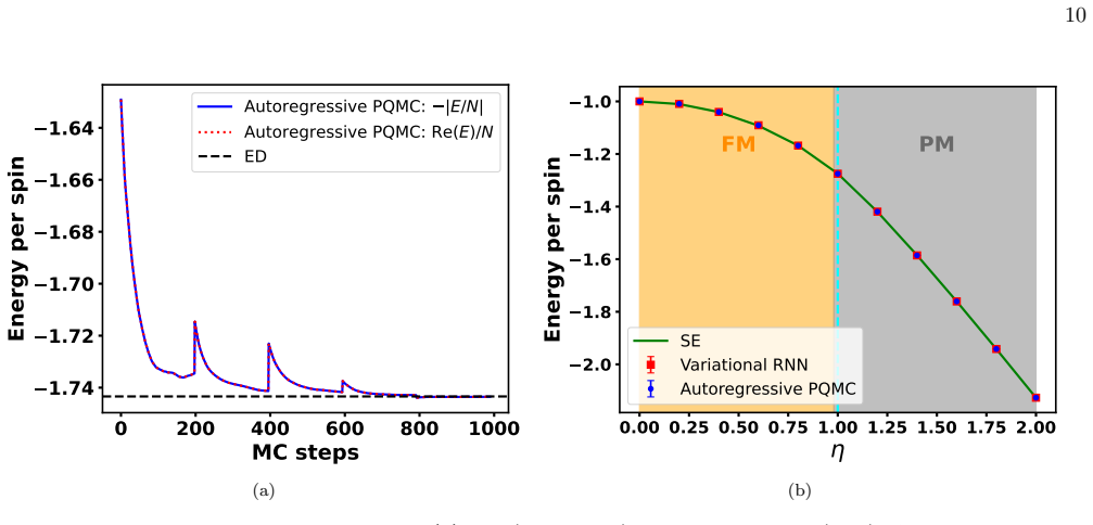
[Appendix C.4, Eqs. (C6)-(C7)] The real-imaginary decomposition used for the non-Hermitian results generates walkers exclusively from H_eta = -J\sum \sigma^z\sigma^z - \eta\sum \sigma^x; the term i\xi D never enters the stochastic dynamics. The self-learning loop therefore converges to a guide proportional to \psi_0(H_eta), and the mixed estimator on that ensemble equals E_0(H_eta) plus i\xi\langle D\rangle_{H_eta}, not the ground-state energy of H = H_eta + i\xi D. For PBCs \langle D\rangle = 0 by one-site translation symmetry; for OBCs the real part is still E_0(H_eta) because \langle D\rangle is real. Hence Figs. 9-10 do not demonstrate PQMC for the non-Hermitian Hamiltonian Eq. (13), and the abstract's "regardless ... non-Hermitian" claim is unsupported. In addition, the manuscript never reports the value of \xi used in any simulation, so the non-Hermitian results cannot be reproduced or checked.
[Appendix C.1, Eq. (C1)] The gauge-rotation argument is incorrect for generic complex g. For a spin flip at site j, the two off-diagonal matrix elements acquire opposite phases, so after the rotation they are of the form -g e^{i\delta} and -g e^{-i\delta}. Both can be real and non-positive only if arg(g) is a multiple of \pi/2; for g = \eta + i\xi with \eta,\xi \neq 0 the transformed pair is complex, and the sign problem is not removed. The text itself notes that one direction gives -|g|e^{\pm 2i\phi}, which is complex, and the subsequent assertion that the Hamiltonian "becomes stoquastic" is therefore not established. This invalidates the stoquasticization claim made in Sec. III.B and Sec. V.A.
[Sec. III.A and Appendix B] The central claim that the self-learning loop is unbiased and that s=5 stints suffice is not supported by a fixed-point analysis. Appendix B only shows energy-per-stint curves for two models, and in the non-Hermitian case those curves are generated by the H_eta walk (see the major comment on Appendix C.4), so they cannot validate convergence to the ground state of Eq. (13). The authors should either prove or numerically demonstrate that the KL-fitted normalized autoregressive distribution converges to \psi_0 rather than to a biased fixed point, and should state an explicit stopping criterion for the number of stints s.

minor comments (5)

[Sec. III.A] The text says that PQMC produces "an updated walker distribution approximating |\psi_0|^2", but the importance-sampled distribution in Eq. (6) is f(x,\tau) = \psi_T(x)\psi(x,\tau), which equals \psi_T\psi_0 only in the \tau\to\infty limit; the training target should be stated consistently with Eq. (6).
[Sec. V.B, Eq. (14)] Equation (14) writes the local energy with the exact right ground-state wavefunction \Psi_{0,R}; in the algorithm the guide is always the current RNN ansatz, so the conditions under which the biorthogonal mixed estimator with an approximate guide equals the non-Hermitian ground-state energy should be stated explicitly.
[Fig. 9 caption] The caption contains "doted line" (should be "dotted line") and "spontaneously PT-unbroken regime" (should be "PT-unbroken regime").
[Appendix D, Table II] The hyperparameter table does not list the value of \xi (or the complex field g = \eta + i\xi) used for the non-Hermitian simulations; without this value the results in Figs. 9-10 are not reproducible.
[Appendix C.1] In the sentence "By the bipartite structure ... the Hamiltonian becomes stoquastic in the later case", the phrase should be "in the latter case", and the sentence is internally contradictory because the preceding expression includes the complex factor e^{\pm 2i\phi}.

Circularity Check

1 steps flagged · score 4.0 of 10

Hermitian benchmark is independent; the NH branch's real-imaginary decomposition (App. C.4) defines the stochastic walk entirely through H_eta, so its 'non-Hermitian' output reduces to a Hermitian H_eta ground state by construction.

self definitional [Appendix C.4, after Eqs. (C6)-(C7)]
"the branching and diffusion Green's function, the single-flip probability Pf and the flip-site selection can be constructed entirely from H_eta. ... the operator i xi D never enters the walker dynamics, the escape rate or the branching weights. Its expectation value is instead accumulated as an additional contribution to the local-energy estimator... This procedure amounts to sampling the ground state of the manifestly stoquastic Hermitian Hamiltonian H_eta via standard PQMC, and evaluating <i xi D> as a mixed estimator on that ensemble, rather than projecting the full NH Hamiltonian."

By the paper's own decomposition (Eq. C7), H = H_eta + i xi D, and all PQMC dynamics are generated from H_eta alone. The importance-sampled walk therefore projects with H_eta, so the self-learning fixed point has the RNN guide approximating psi_0(H_eta), not psi_0(H). The reported energy is then <psi_0(H_eta)|H|psi_0(H_eta)>/<psi_0(H_eta)|psi_0(H_eta)> = E_0(H_eta) + i xi <D>_0. Since H_eta is a uniform-field transverse-field Ising model, its ground state is translation invariant and <D>_0 = 0, so the 'non-Hermitian' result is simply E_0(H_eta), independent of xi.

full rationale

The Hermitian core of the paper is self-contained: Eq. (9) is benchmarked against an independent Jordan-Wigner-Bogoliubov solution and exact diagonalization (Fig. 5, Table I), and the RNN-guided PQMC energy is a stochastic mixed estimator of H, not a parameter fitted to the benchmark. The self-learning loop in Sec. III.A trains the RNN to the PQMC walker distribution, but the final energy still comes from the PQMC local-energy estimator, so no fitted parameter is relabeled as a prediction. The comparison with the variational RNN from Ref. [20] is a self-citation, but it is not load-bearing because ED and high-order series expansions [52] independently anchor the energies. The substantive circularity risk is in the non-Hermitian branch: Appendix C.4 explicitly constructs all stochastic dynamics from the Hermitian H_eta part and only appends <i xi D> as a mixed estimator on that H_eta ensemble. At the self-learning fixed point the guide is fit to H_eta, not to H, making the reported 'non-Hermitian' energy E_0(H_eta) + i xi <D> with <D> = 0 by symmetry; the xi-dependence, and with it the claimed non-Hermitian performance, is an input of the algorithm rather than a derived prediction. Since the paper does not report the imaginary coupling xi used in any NH benchmark nor state which appendix method produced Figs. 9-10, this construction-level reduction is not resolved. Overall, the Hermitian derivation is not circular, but the central 'regardless ... non-Hermitian' claim rests on a branch that reduces to a Hermitian H_eta calculation by construction.

Assumptions & free parameters 2 free parameters · 3 assumptions · 1 invented entities

The central claim rests on the convergence of the self-learning loop (an assumed property, not proven), on the applicability of PQMC to stoquastic-transformed NH Hamiltonians (a domain assumption the authors state may fail for arbitrary NH models), and on the quality of the RNN guide for the NH real-imaginary decomposition. The free parameters are algorithm choices (time step, regulator) rather than physics parameters. No genuinely new physical entity is introduced.

free parameters (2)

Time step dt = 10^-2 (and range 10^-1 to 10^-5 in Table II)
Chosen by hand; bias is mitigated by continuous-time PQMC, but the finite-dt bias is assessed by fitting the error curves in Fig. 2. The choice affects the results but is a standard algorithmic parameter.
Reference energy regulator mu = Not reported numerically, described as a small positive factor
Used in E_r = E + mu log(N_avg/N_cur) to control the walker population; its value is not given in Table II.

assumptions (3)

ad hoc to paper The self-learning PQMC loop converges to the true ground state when the RNN guide is trained on walker configurations by KL divergence minimization.
Section III.A asserts convergence when s tends to infinity and that s=5 stints suffice, but no unbiasedness or convergence proof is provided. The method's central claim depends on this.
domain assumption PQMC is applicable to the non-Hermitian Hamiltonian after a gauge rotation makes it stoquastic.
Appendix C.1 constructs the gauge rotation and states the rotated Hamiltonian becomes stoquastic. The paper explicitly warns that this is not a general framework and may fail for arbitrary NH Hamiltonians.
ad hoc to paper The real-imaginary decomposition for the NH model yields an unbiased estimate of the complex local energy when the guide is good.
Appendix C.4 states the procedure 'amounts to sampling the ground state of the manifestly stoquastic Hermitian Hamiltonian H_eta' and that it is 'exact when the guiding wavefunction is a sufficiently good approximation.' This is an unverified assumption.

invented entities (1)

Gauge-rotated stoquastic Hamiltonian H_rot
purpose: Makes the complex off-diagonal elements of the non-Hermitian Ising chain real and non-positive, avoiding the sign problem.
This is a basis choice for the same Hamiltonian, not a new physical entity. It has no independent falsifiable handle outside the paper.

how reviews work

0 comments

Cite this review

Pith. "Pith review of Autoregressive Projective Quantum Monte Carlo: From a Hermitian to a Non-Hermitian Perspective." pith.science (2026). https://pith.science/paper/HOUWECPM

@misc{pith2026260809496,
  author       = {Pith},
  title        = {Pith review of: Autoregressive Projective Quantum Monte Carlo: From a Hermitian to a Non-Hermitian Perspective},
  year         = {2026},
  howpublished = {\url{https://pith.science/paper/HOUWECPM}},
  note         = {Machine review of arXiv:2608.09496}
}

read the original abstract

Accurately determining the ground-state properties of quantum many-body systems remains a central challenge. In this work, we introduce an autoregressive projective quantum Monte Carlo (PQMC) framework that leverages recurrent neural networks (RNNs) to guide the stochastic dynamics. By incorporating autoregressive sampling into PQMC, we demonstrate substantial improvements in accuracy compared to standard unguided PQMC, while retaining polynomial computational cost. We benchmark our approach against conventional variational RNN ans\"atze and find that the autoregressive PQMC consistently achieves lower energies and higher fidelity, regardless of system size or whether the Hamiltonian is Hermitian or non-Hermitian. Our results highlight the versatility and power of neural-guided PQMC methods, paving the way for promising scalable simulations of low-energy states in complex quantum many-body systems.

Figures

Figures reproduced from arXiv: 2608.09496 by the authors.

**Figure 1.** PQMC guided by an NQS. We represent a simplified schematic plot of the PQMC guided by an NQS. Here, the NQS uses the set of walkers {x} from the PQMC to train an ansatz ψ, which should be a “good” approximation of the target ground state. This ansatz is then used to guide the PQMC simulation and to compute the local energies Eloc. The ground state energy is obtained by averaging these local energies. systems–a regim… view at source ↗

**Figure 2.** Bias due to time step. The relative error εrel is plotted against the imaginary time step ∆τ for the continuous-time PQMC (blue), symmetrized SPQMC (red), and non-symmetrized SPQMC (purple). The simulation is performed for Nw = 103 walkers, and N = 20 spins. For continuous-time PQMC, a blue line is provided to guide the eye, as fitting is not meaningful in this case. The symmetrized SPQMC curve is fitted with a quad… view at source ↗

**Figure 3.** Autoregressive PQMC. We show a schematic plot of self-learning PQMC guided by an RNN. θ are the RNN parameters. C. Continuous Time Approximation First introduced in Refs. [31–33], the idea behind the continuous-time approximation is to slice the MC time step ∆τ into m → ∞ small intervals, extract the time δτp that passes before the transition to the next configuration, and keep track of the remaining time δτr neede… view at source ↗

Figures from the paper (9 more)

**Figure 4.** Figure 4: Hermitian 1D Ising chain with alternating magnetic field. A (red) and B (blue) represent the sublattices in which spin-1/2 particles occupy the odd and even positions, respectively. The transverse field +g (−g) is applied to the B (A) sublattices. Nearest-neighbor coup…

**Figure 5.** Figure 5: Autoregressive PQMC vs SPQMC and ED. We plot (a) the energy per spin with SPQMC (red), and PQMC using a random ψT (green) for ∆τ = 10−2 , g = 1.6, Nw = 2 × 104 , MCs = 2 × 103 , and the projection time ∆τp = MCs × ∆τ = 20. The energy per spin obtained using autoregress…

**Figure 6.** Figure 6: Relative errors. We plot the relative error εrel on the energy with respect to ED as a function of (a) the field strength g using SPQMC (red) and neural-guided autoregressive PQMC (blue) for ∆τ = 10−2 , Nw = 2 × 104 , MCs = 2 × 103 , projection time ∆τp = MCs × ∆τ = 20…

**Figure 8.** Figure 8: Non-Hermitian 1D Ising chain in a staggered magnetic field. A (red) and B (blue) represent the sublattices in which spin-1/2 particles occupy the odd and even positions, respectively. The complex field g (g ∗ ) is applied to the A (B) sublattices [20]. Nearest-neighbor…

**Figure 7.** Figure 7: Phase diagram. Ground-state energy per spin for both the ferromagnetic (FM, orange background) and paramagnetic (PM, gray) regimes for N = 20 spins. Both methods are in good agreement with ED and JWB methods. PBCs are considered. blue) converges to a lower variance tha…

**Figure 9.** Figure 9: Energy per spin. We compute the (a) real (red dashed) and absolute value (blue) of the ground-state energy per spin using autoregressive PQMC and benchmark against ED (black dashed) for N = 10. (b) Phase diagram: energy per spin as a function of the real part of the fi…

**Figure 10.** Figure 10: Relative error. Relative error achieved with variational RNN (purple) and autoregressive PQMC (blue) as a function of system size. OBCs are considered. The autoregressive PQMC exhibits slower scaling and a lower relative error in the energy with increasing system size…

**Figure 11.** Figure 11: Energy per stint. We plot the energy per spin per stint −⟨E/N⟩s for the (a) Hermitian, and (b) non-Hermitian Ising chain. We consider N = 20 and N = 10, respectively. We observe that the autoregressive PQMC (in blue) is more accurate after each stint finally convergin…

**Figure 12.** Figure 12: Variational RNN versus SPQMC versus autoregressive PQMC. We compare the variational RNN (RNN with VMC) with the autoregressive PQMC. We see that the later (blue) achieves less error than the variational RNN (purple), which is also less accurate than SPQMC (red). We co…

Discussion (0). Continue with ORCID to comment.

Reference graph

Works this paper leans on

57 extracted references · 42 canonical work pages

[1]

sign problem

Gauge rotation In quantum Monte Carlo (VMC, PQMC,...), one sam- ples spin configurationsxwith a positive definite weight ω(x). In the computational basisσ z, the off-diagonal matrix elements⟨x ′∣H∣x⟩of our non-Hermitian Ising chain are complex, leading to complex weightsω(x). As a result, the variance of observables grows exponen- tially with system size,...

work page
[2]

In principle, for a NH system in aP T-unbroken regime, one can always find a simi- larity transformation that transforms the model into a Hermitian model [48]

Similarity transform In addition to the gauge rotation, one could also use a similarity transformation [48, 49] to mitigate the sign problem in NH systems. In principle, for a NH system in aP T-unbroken regime, one can always find a simi- larity transformation that transforms the model into a Hermitian model [48]. For aP T-symmetric HamiltonianHin the unb...

work page
[3]

Gauge rotation vs similarity transform: The nonlocality While mathematically elegant, we argue that the simi- larity transform has some practical challenges compared to the gauge rotation method. First, in some cases, the metric operator is constructed from the outer product of the biorthogonal eigenpairs, and necessitates knowledge of all the eigenstates...

work page
[4]

closed-form

Real-imaginary decomposition In addition to the two previously proposed methods, one could use the so-called real-imaginary decomposi- tion, where the idea is to perform a mixed estimator and perturbative treatment ofξrather than an exact non- Hermitian projection. While relatively simpler than the two previous methods, is method is also restricted to onl...

work page
[5]

J. B. Anderson, A random-walk simulation of the schr¨ odinger equation: H+ 3, The Journal of Chemical Physics63, 1499 (1975)

work page 1975
[6]

P. J. Reynolds, D. M. Ceperley, B. J. Alder, and W. A. Lester Jr, Fixed-node quantum monte carlo for molecules, The Journal of Chemical Physics77, 5593 (1982)

work page 1982
[7]

von der Linden, A quantum monte carlo approach to many-body physics, Physics Reports220, 53 (1992)

W. von der Linden, A quantum monte carlo approach to many-body physics, Physics Reports220, 53 (1992)

work page 1992
[8]

B. G. A. Brito, G.-Q. Hai, and L. Cˆ andido, Quantum monte carlo simulation for the many-body decomposi- tion of the interaction energy and electron correlation of small superalkali lithium clusters, The Journal of Chem- ical Physics151, 014303 (2019)

work page 2019

Show all 57 references

[9]

D. M. Ceperley and B. J. Alder, Ground state of the elec- tron gas by a stochastic method, Physical review letters 45, 566 (1980)

1980
[10]

Sprague and S

K. Sprague and S. Czischek, Variational monte carlo with large patched transformers, Communications Physics7, 90 (2024)

2024
[11]

Ceperley, G

D. Ceperley, G. V. Chester, and M. H. Kalos, Monte carlo simulation of a many-fermion study, Physical Review B 16, 3081 (1977)

1977
[12]

Herman, E

M. Herman, E. Bruskin, and B. Berne, On path inte- gral monte carlo simulations, The Journal of Chemical Physics76, 5150 (1982)

1982
[13]

E. M. Inack, G. E. Santoro, and S. Pilati,Simulating quantum annealing viaprojective quantum Monte Carloal- gorithms, Ph.D. thesis, SISSA (2017)

2017
[14]

Kr¨ amer, J

C. Kr¨ amer, J. A. Koziol, A. Langheld, M. H¨ ormann, and K. P. Schmidt, Quantum-critical properties of the one- and two-dimensional random transverse-field ising model from large-scale quantum monte carlo simulations, Sci- Post Physics17, 061 (2024)

2024
[15]

D. M. Ceperley, Path integrals in the theory of condensed helium, Reviews of Modern Physics67, 279 (1995)

1995
[16]

E. M. Inack and S. Pilati, Simulated quantum annealing of double-well and multiwell potentials, Phys. Rev. E92, 053304 (2015)

2015
[17]

Carlo, Diffusion quantum monte carlo, Computers in Physics4, 662 (1990)

M. Carlo, Diffusion quantum monte carlo, Computers in Physics4, 662 (1990)

1990
[18]

Pilati, E

S. Pilati, E. Inack, and P. Pieri, Self-learning projective quantum monte carlo simulations guided by restricted boltzmann machines, Physical Review E100, 043301 (2019)

2019
[19]

Feldbacher, K

M. Feldbacher, K. Held, and F. F. Assaad, Projective quantum monte carlo method for the anderson impurity model and its application to dynamical mean field the- ory., Physical review letters93 13, 136405 (2004)

2004
[20]

R. G. Parr, Density functional theory, inElectron Dis- tributions and the Chemical Bond(Springer, 1982) pp. 95–100

1982
[21]

Isozaki, Many-body schr¨ odinger equation, Springer, Tokyo https://doi.org/10.1007/978-981-99-3704-2 (2004)

H. Isozaki, Many-body schr¨ odinger equation, Springer, Tokyo https://doi.org/10.1007/978-981-99-3704-2 (2004)

2004 doi
[22]

N. H. March, W. H. Young, and S. Sampanthar,The many-body problem in quantum mechanics(Courier Cor- poration, 1995). 17

1995
[23]

Neklyudov, J

K. Neklyudov, J. Nys, L. Thiede, J. Carrasquilla, Q. Liu, M. Welling, and A. Makhzani, Wasserstein quantum monte carlo: a novel approach for solving the quantum many-body schr¨ odinger equation, Advances in Neural In- formation Processing Systems36(2024)

2024
[24]

L. Wah, R. Zen, and F. K. Kunst, Many-body neural network wavefunction for a non-hermitian ising chain, Phys. Rev. Res.7, 043291 (2025)

2025
[25]

Hibat-Allah, M

M. Hibat-Allah, M. Ganahl, L. E. Hayward, R. G. Melko, and J. Carrasquilla, Recurrent neural network wave func- tions, Physical Review Research2, 023358 (2020)

2020
[26]

Carleo and M

G. Carleo and M. Troyer, Solving the quantum many- body problem with artificial neural networks, Science 355, 602 (2017)

2017
[27]

Carrasquilla and G

J. Carrasquilla and G. Torlai, How to use neural net- works to investigate quantum many-body physics, PRX Quantum2, 040201 (2021)

2021
[28]

J. Kim, G. Pescia, B. Fore, J. Nys, G. Carleo, S. Gan- dolfi, M. Hjorth-Jensen, and A. Lovato, Neural-network quantum states for ultra-cold fermi gases, Communica- tions Physics7, 148 (2024)

2024
[29]

L. Wah, F. K. Kunst, and M. Hibat-Allah, Bridging frustration and non-hermiticity via compass: An adap- tive biorthogonal neural quantum state framework, arXiv preprint arXiv:2607.13790 (2026)

2026 arXiv
[30]

Sorella, Wave function optimization in the variational monte carlo method, Physical Review B—Condensed Matter and Materials Physics71, 241103 (2005)

S. Sorella, Wave function optimization in the variational monte carlo method, Physical Review B—Condensed Matter and Materials Physics71, 241103 (2005)

2005
[31]

Solinas, B

M. Solinas, B. Barton, Y. Zhang, J. Nys, and J. Car- rasquilla, Biorthogonal neural network approach to two-dimensional non-hermitian systems, arXiv preprint arXiv:2508.01072 (2025)

2025
[32]

Zhang, J

S. Zhang, J. Carlson, and J. E. Gubernatis, Constrained path quantum monte carlo method for fermion ground states, Phys. Rev. Lett.74, 3652 (1995)

1995
[33]

Feldbacher, K

M. Feldbacher, K. Held, and F. F. Assaad, Projective quantum monte carlo method for the anderson impurity model and its application to dynamical mean field theory, Phys. Rev. Lett.93, 136405 (2004)

2004
[34]

R. M. Fye, New results on trotter-like approximations, Phys. Rev. B33, 6271 (1986)

1986
[35]

Sorella, Green function monte carlo with stochastic reconfiguration, Physical review letters80, 4558 (1998)

S. Sorella, Green function monte carlo with stochastic reconfiguration, Physical review letters80, 4558 (1998)

1998
[36]

Sorella and L

S. Sorella and L. Capriotti, Green function monte carlo with stochastic reconfiguration: An effective remedy for the sign problem, Physical Review B61, 2599 (2000)

2000
[37]

Becca and S

F. Becca and S. Sorella,Quantum Monte Carlo ap- proaches for correlated systems(Cambridge University Press, 2017)

2017
[38]

D. Luo, Z. Chen, J. Carrasquilla, and B. K. Clark, Au- toregressive neural network for simulating open quantum systems via a probabilistic formulation, Phys. Rev. Lett. 128, 090501 (2022)

2022
[39]

Fischer and C

A. Fischer and C. Igel, Empirical analysis of the di- vergence of gibbs sampling based learning algorithms for restricted boltzmann machines, inArtificial Neural Networks – ICANN 2010, edited by K. Diamantaras, W. Duch, and L. S. Iliadis (Springer Berlin Heidelberg, Berlin, He...

2010
[40]

Kullback, Kullback-leibler divergence, Tech

S. Kullback, Kullback-leibler divergence, Tech. Rep. (1951)

1951
[41]

L. Jiao, X. Song, C. You, X. Liu, L. Li, P. Chen, X. Tang, Z. Feng, F. Liu, Y. Guo,et al., Ai meets physics: a com- prehensive survey, Artificial Intelligence Review57, 256 (2024)

2024
[42]

Sharir, Y

O. Sharir, Y. Levine, N. Wies, G. Carleo, and A. Shashua, Deep autoregressive models for the efficient variational simulation of many-body quantum systems, Phys. Rev. Lett.124, 020503 (2020)

2020
[43]

R. G. Melko, G. Carleo, J. Carrasquilla, and J. I. Cirac, Restricted boltzmann machines in quantum physics, Na- ture Physics15, 887 (2019)

2019
[44]

Rautela, A

M. Rautela, A. Williams, and A. Scheinker, A conditional latent autoregressive recurrent model for generation and forecasting of beam dynamics in particle accelerators, Scientific Reports14, 18157 (2024)

2024
[45]

T. A. Kumar, L. Balents, T. H. Hsieh, and R. G. Melko, Autoregressive typical thermal states, arXiv preprint arXiv:2508.13455 (2025)

2025 arXiv
[46]

Parthipan, H

R. Parthipan, H. M. Christensen, J. S. Hosking, and D. J. Wischik, Using probabilistic machine learning to better model temporal patterns in parameterizations: a case study with the lorenz 96 model, Geoscientific Model De- velopment16, 4501 (2023)

2023
[47]

Loh Jr, J

E. Loh Jr, J. Gubernatis, R. Scalettar, S. White, D. Scalapino, and R. Sugar, Sign problem in the numeri- cal simulation of many-electron systems, Physical Review B41, 9301 (1990)

1990
[48]

G. H. Booth, A. J. Thom, and A. Alavi, Fermion monte carlo without fixed nodes: A game of life, death, and annihilation in slater determi- nant space, The Journal of chemical physics131, https://doi.org/10.1063/1.3193710 (2009)

2009 doi
[49]

Ceperley and B

D. Ceperley and B. Alder, Quantum monte carlo for molecules: Green’s function and nodal release, The Jour- nal of chemical physics81, 5833 (1984)

1984
[50]

Y. Mori, K. Kashiwa, and A. Ohnishi, Toward solving the sign problem with path optimization method, Physical Review D96, 111501 (2017)

2017
[51]

Li, Y.-F

Z.-X. Li, Y.-F. Jiang, and H. Yao, Solving the fermion sign problem in quantum monte carlo simulations by majorana representation, Physical Review B91, 241117 (2015)

2015
[52]

Mostafazadeh, Exact pt-symmetry is equivalent to hermiticity, Journal of Physics A: Mathematical and General36, 7081 (2003)

A. Mostafazadeh, Exact pt-symmetry is equivalent to hermiticity, Journal of Physics A: Mathematical and General36, 7081 (2003)

2003
[53]

Miao and Z.-M

Y.-G. Miao and Z.-M. Xu, Investigation of non-hermitian hamiltonians in the heisenberg picture, Physics Letters A 380, 1805 (2016)

2016
[54]

E. Lieb, T. Schultz, and D. Mattis, Two soluble models of an antiferromagnetic chain, Annals of Physics16, 407 (1961)

1961
[55]

E. J. Bergholtz, J. C. Budich, and F. K. Kunst, Ex- ceptional topology of non-hermitian systems, Rev. Mod. Phys.93, 015005 (2021)

2021
[56]

Lenke, M

L. Lenke, M. M¨ uhlhauser, and K. P. Schmidt, High-order series expansion of non-hermitian quantum spin models, Phys. Rev. B104, 195137 (2021)

2021
[57]

C. M. Bender, Introduction to pt-symmetric quantum theory, Contemporary physics46, 277 (2005)

2005

Pith tools

Reviewed August 11, 2026 · model on record in the stance chip above.

[1] [1]

sign problem

Gauge rotation In quantum Monte Carlo (VMC, PQMC,...), one sam- ples spin configurationsxwith a positive definite weight ω(x). In the computational basisσ z, the off-diagonal matrix elements⟨x ′∣H∣x⟩of our non-Hermitian Ising chain are complex, leading to complex weightsω(x). As a result, the variance of observables grows exponen- tially with system size,...

work page

[2] [2]

In principle, for a NH system in aP T-unbroken regime, one can always find a simi- larity transformation that transforms the model into a Hermitian model [48]

Similarity transform In addition to the gauge rotation, one could also use a similarity transformation [48, 49] to mitigate the sign problem in NH systems. In principle, for a NH system in aP T-unbroken regime, one can always find a simi- larity transformation that transforms the model into a Hermitian model [48]. For aP T-symmetric HamiltonianHin the unb...

work page

[3] [3]

Gauge rotation vs similarity transform: The nonlocality While mathematically elegant, we argue that the simi- larity transform has some practical challenges compared to the gauge rotation method. First, in some cases, the metric operator is constructed from the outer product of the biorthogonal eigenpairs, and necessitates knowledge of all the eigenstates...

work page

[4] [4]

closed-form

Real-imaginary decomposition In addition to the two previously proposed methods, one could use the so-called real-imaginary decomposi- tion, where the idea is to perform a mixed estimator and perturbative treatment ofξrather than an exact non- Hermitian projection. While relatively simpler than the two previous methods, is method is also restricted to onl...

work page

[5] [5]

J. B. Anderson, A random-walk simulation of the schr¨ odinger equation: H+ 3, The Journal of Chemical Physics63, 1499 (1975)

work page 1975

[6] [6]

P. J. Reynolds, D. M. Ceperley, B. J. Alder, and W. A. Lester Jr, Fixed-node quantum monte carlo for molecules, The Journal of Chemical Physics77, 5593 (1982)

work page 1982

[7] [7]

von der Linden, A quantum monte carlo approach to many-body physics, Physics Reports220, 53 (1992)

W. von der Linden, A quantum monte carlo approach to many-body physics, Physics Reports220, 53 (1992)

work page 1992

[8] [8]

B. G. A. Brito, G.-Q. Hai, and L. Cˆ andido, Quantum monte carlo simulation for the many-body decomposi- tion of the interaction energy and electron correlation of small superalkali lithium clusters, The Journal of Chem- ical Physics151, 014303 (2019)

work page 2019