The WDM Time-Frequency Transform in Gravitational-Wave Data Analysis I: Formalism
Pith reviewed 2026-06-26 13:26 UTC · model grok-4.3
The pith
The WDM basis supplies orthogonal functions with good time-frequency localization for gravitational-wave analysis when noise varies slowly.
A machine-rendered reading of the paper's core claim, the machinery that carries it, and where it could break.
Core claim
The paper establishes that the WDM basis provides a complete set of orthogonal functions with controlled time-frequency support, allowing direct derivation of the forward and inverse transforms, explicit handling of edge effects at DC and Nyquist frequencies, and construction of the time-frequency domain likelihood from the noise covariance when detector noise varies slowly.
What carries the argument
The Wilson-Daubechies-Meyer (WDM) basis, a collection of orthogonal functions engineered for simultaneous localization in time and frequency.
If this is right
- The forward and inverse transforms admit direct numerical implementation with documented edge-effect corrections.
- The noise covariance matrix in the time-frequency domain is determined by the slow-variation assumption alone.
- The likelihood function can be written and evaluated entirely inside the time-frequency representation.
- Analysts obtain a concrete middle option between frequency-domain speed and time-domain flexibility for signals embedded in slowly evolving noise.
Where Pith is reading between the lines
- The same orthogonality and localization properties could be checked for other bases before adopting them in similar pipelines.
- The covariance construction may extend to piecewise-slow noise models by stitching adjacent time-frequency tiles.
- Parameter estimation codes could replace their frequency-domain likelihood module with the derived time-frequency version without altering the rest of the sampling machinery.
Load-bearing premise
Detector noise varies slowly enough that a time-frequency representation sits between frequency-domain efficiency and time-domain generality.
What would settle it
A calculation showing that the time-frequency likelihood produces systematically different posterior distributions from the frequency-domain likelihood on the same data with slowly varying noise would falsify the claimed practical advantage.
Figures

read the original abstract
For slowly-varying noise, time-frequency methods offer a natural middle ground between the efficiency of the frequency domain and the generality of the more expensive time domain. Despite growing adoption, such methods remain less well documented and less familiar in the gravitational-wave literature, compared to the ubiquitous frequency domain. Aimed at gravitational-wave analysts, in this paper we present a self-contained account of time-frequency methods, detail derivations for a specific basis, namely the Wilson-Daubechies-Meyer (WDM) basis, and share intuition and lessons learned. We document key concepts: the orthogonality and good time-frequency localization of the basis, the edge effects at the DC and Nyquist frequencies, the forward and inverse transforms and their practical implementation, and the noise covariance matrix and likelihood in the time-frequency domain.
Editorial analysis
A structured set of objections, weighed in public.
Referee Report
Summary. The paper provides a self-contained formal account of time-frequency methods for gravitational-wave data analysis under slowly-varying noise, with explicit derivations for the Wilson-Daubechies-Meyer (WDM) basis. It covers the orthogonality and time-frequency localization properties of the basis, edge effects at DC and Nyquist frequencies, the forward and inverse transforms with practical implementation details, and the construction of the noise covariance matrix and likelihood function in the time-frequency domain.
Significance. If the derivations hold, the work fills a documentation gap in the GW literature by making time-frequency techniques more accessible and reproducible, serving as a reference that bridges the efficiency of frequency-domain methods with the flexibility needed for non-stationary noise. The explicit treatment of the likelihood and covariance under the slowly-varying assumption strengthens its utility for practical data analysis pipelines.
minor comments (2)
- The abstract states that 'lessons learned' are shared, but the manuscript would benefit from a dedicated subsection or table summarizing practical implementation pitfalls (e.g., numerical stability at boundaries) to make this aspect more prominent for readers.
- Notation for the WDM basis functions and their duals should be introduced with a clear comparison table to other common bases (e.g., short-time Fourier transform) early in the text to aid readers new to the formalism.
Simulated Author's Rebuttal
We thank the referee for their positive assessment of the manuscript and for recommending acceptance. We appreciate the recognition that the work provides a self-contained formal account of time-frequency methods and fills a documentation gap in the gravitational-wave literature.
Circularity Check
No significant circularity detected
full rationale
The paper explicitly frames itself as a self-contained documentation of the WDM basis, deriving orthogonality, time-frequency localization, forward/inverse transforms, edge handling, and the time-frequency likelihood from standard basis properties under the slowly-varying noise condition. No load-bearing step reduces by construction to a fitted input, self-definition, or self-citation chain; the derivations are presented as independent formal steps from established wavelet properties. This matches the default expectation of a non-circular formal exposition.
Axiom & Free-Parameter Ledger
axioms (1)
- domain assumption Detector noise is slowly-varying
Reference graph
Works this paper leans on
-
[1]
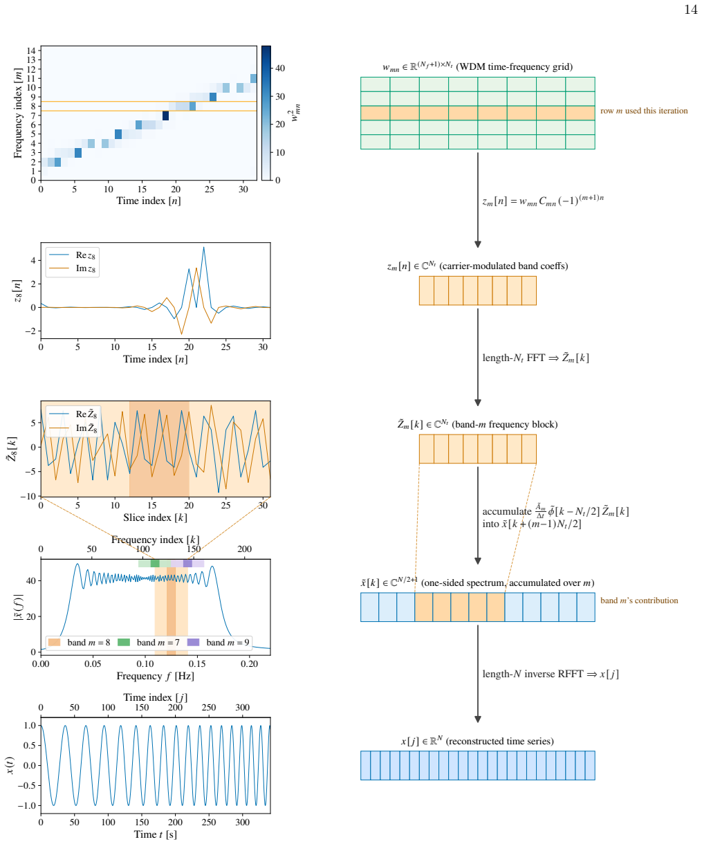
We now switch to practical implementation details and discretize it, also switching from the FFT convention of Eq
Discretization Equation (28) gives the WDM coefficients for the continuous transform. We now switch to practical implementation details and discretize it, also switching from the FFT convention of Eq. (4) to thenumpydiscrete Fourier transform of Eq. (6). The discretizationf k =k∆fhas two effects: (i) ˜x(f k)→∆t˜x[k], and (ii) the WDM integral becomes a su...
-
[2]
(39) drops out as ˜ϕ(f+m∆F) has no support forf >0
Interior frequency Bands For the interior bands,m̸= 0, N f, the first term of Eq. (39) drops out as ˜ϕ(f+m∆F) has no support forf >0. The contribution of a single interior bandmon the frequency-domain data is ˜xm(f) = 1√ 2 Nt−1X n=0 wmnCmne−2πinf∆T ˜ϕ(f−m∆F).(40) Transformingf ′ =f−m∆F(and relabelingf ′ →f) yields ˜xm (f+m∆F) = 1√ 2 ˜ϕ(f) Nt−1X n=0 wmnCmn...
-
[3]
The two terms in the square bracket of Eq
Edge frequency bands The contribution of the edge bandsm= 0, N f requires two modifications: the basis prefactor is 1/2 instead of 1/ √ 2 and the positive/negative components of the basis coincide. The two terms in the square bracket of Eq. (39) collapse to a single filter, which follows immediately form= 0 and by the arguments of Appendix C for the 2f Ny...
-
[4]
The factor of √ 2 is a combination of two effects: (i) division by √ 2 to account for the different basis prefactor, but also (ii) multiplication by 2 for the coinciding positive/negative frequency filters. 13
-
[5]
To cover all bands with a single equation, we define ˜Am = 1/(2Am) instead of the basis prefactor for the interior or exterior bands
Discretization To discretize, we setf k =k∆fand ˜x m(f)→∆t˜x m[k]. To cover all bands with a single equation, we define ˜Am = 1/(2Am) instead of the basis prefactor for the interior or exterior bands. Starting with Eq. (41) ∆t˜xm k+m Nt 2 = ˜Am ˜ϕ[k] Nt−1X n=0 (−1)mnwmnCmne−2πink/Nt .(44) Following similar steps to the forward transform, we center the fil...
-
[6]
Z (m′+1)∆F (m′−1)∆F Z (m+1)∆F (m−1)∆F Cm′n′C ∗ mnS(f)δ(f−f ′)˜ϕ(f−m∆F) ˜ϕ(f ′ −m ′∆F)e 2πi(nf−n ′f ′)∆T dfdf ′ # =A mAm′ℜ
Forward transform Returning to Eq. (55), we start with the first term, I XY (mn)(m′n′) = 2AmAm′ Z (m′+1)∆F (m′−1)∆F Z (m+1)∆F (m−1)∆F ℜ ⟨X(f)Y(f ′)⟩dfdf ′ =A mAm′ℜ "Z (m′+1)∆F (m′−1)∆F Z (m+1)∆F (m−1)∆F Cm′n′C ∗ mnS(f)δ(f−f ′)˜ϕ(f−m∆F) ˜ϕ(f ′ −m ′∆F)e 2πi(nf−n ′f ′)∆T dfdf ′ # =A mAm′ℜ " Cm′n′C ∗ mn Z (m+1)∆F (m−1)∆F S(f) ˜ϕ(f−m∆F) ˜ϕ(f−m ′∆F)e 2πi(n−n′)f...
-
[7]
˜A2 m ˜ϕ2(f−m∆F) X r tmm[r]e−2πif r∆T + 2ℜ ˜Am ˜Am+1 ˜ϕ(f−m∆F) ˜ϕ(f−(m+ 1)∆F) X r tmm+1[r]e−2πif r∆T # . (76) and after one final translation tof→f+m∆Fwe obtain, Σ= NfX m=0
Inverse transform We now present the inverse transform to return from the WDM domain noise covariance matrix Λ (mn)(m′n′) to the noise PSD in the frequency domainS(f). We start with Eq. (57) and specializing to the stationary noise case, f=f ′, collapses the sumsm, m ′ to only the band-tridiagonalm=m ′ andm=m ′ ±1. Since the covariance matrix is symmetric...
-
[8]
(67), we follow similar steps to Sec
Discretization To discretize the covariance expression for Eq. (67), we follow similar steps to Sec. III A 1:f→k∆f, ˜x(f)→˜x[k], andd f→∆f. The stationary PSD is evaluated at each of the binsm∆F, yielding Λ(mn)(m′n′) = 1 2∆f(−1)(n−n′)m ℜ Cm′n′C ∗ mn Nt/2−1X k=−Nt/2 S k+m Nt 2 ˜ϕ[k] ˜ϕ k+ (m−m ′) Nt 2 e2πi(n−n′)k/Nt . (78) Centering the bins wit...
-
[9]
(81) has (N f + 1)Nt ×(N f + 1)Nt entries that encode theN/2 + 1 degrees of freedom of stationary noise
Structure The noise covariance matrix of Eq. (81) has (N f + 1)Nt ×(N f + 1)Nt entries that encode theN/2 + 1 degrees of freedom of stationary noise. Its structure is simplified by a number of symmetries, but even then the number of nonzero, unique entries is greater thanN/2 + 1. This means that entries are in general not independent even when symmetries ...
-
[10]
The covariance matrix is symmetric in (mn)↔(m ′n′)
-
[11]
It therefore suffices to compute them=m ′ andm=m ′ + 1 elements and obtain them=m ′ −1 entries by symmetry
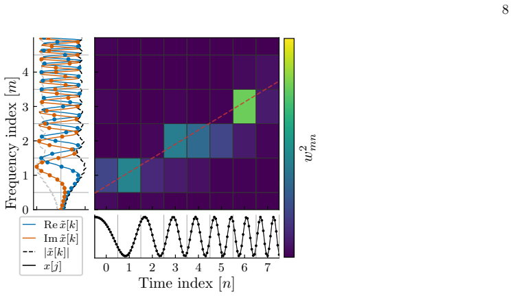
It is block tri-diagonal, where the three diagonals correspond to|m−m ′| ≤1 and the blocks correspond ton. It therefore suffices to compute them=m ′ andm=m ′ + 1 elements and obtain them=m ′ −1 entries by symmetry. 5 ForN t = 4 in particular, all cross-band blocks vanish, but that is not a generic property of otherN t values and hence we do not show it he...
-
[12]
Up to parity each (m, m ′) block depends onn, n ′ only throughr=n−n ′ and therefore has a parity-corrected Toeplitz structure
-
[13]
In our example, this corresponds to blocksD 1 andD 2, each of which is schematically Dm = d0 d1 d2 d3 d1 d0 −d1 d2 d2 −d1 d0 d1 d3 d2 d1 d0 .(88)
The interior (m, m ′ ̸= 0, N f) diagonal (m=m ′) blocks are symmetric, have a constant diagonal, and are Toeplitz forreven and alternating-sign Toeplitz forrodd. In our example, this corresponds to blocksD 1 andD 2, each of which is schematically Dm = d0 d1 d2 d3 d1 d0 −d1 d2 d2 −d1 d0 d1 d3 d2 d1 d0 .(88)
-
[14]
In our example, this corresponds to blocksD 0 andD 3, the former of which is schematically Dm = d0 0d 2 0 0 0 0 0 d2 0d 0 0 0 0 0 0 .(89)
The edge (m, m ′ = 0, Nf) diagonal (m=m ′) blocks have similar properties as the interior ones and additionally rows/columns withm+nodd vanish identically. In our example, this corresponds to blocksD 0 andD 3, the former of which is schematically Dm = d0 0d 2 0 0 0 0 0 d2 0d 0 0 0 0 0 0 .(89)
-
[15]
Overall then,ℜ n CmnC ∗ (m+1)nKm(m+1) o = 0
The diagonal elements of the cross-band blocks vanish by parity arguments: form ′ =m+ 1 andr=n−n ′ = 0, Km(m+1) is purely real, whileC mnC ∗ (m+1)n is purely imaginary. Overall then,ℜ n CmnC ∗ (m+1)nKm(m+1) o = 0
-
[16]
The blocks are not fully symmetric, as odd-rstripes are symmetric and even-rstripes are antisymmetric
The interior (m, m ′ ̸= 0, N f) cross-band (m=m ′ + 1) blocks are Toeplitz forrodd and alternating-sign Toeplitz forreven. The blocks are not fully symmetric, as odd-rstripes are symmetric and even-rstripes are antisymmetric. In our example, this corresponds to blocksB 12 andB 21, each of which is schematically Bm,m+1 = 0b 1 −b2 b3 b1 0b 1 b2 b2 b1 0...
-
[17]
mother wavelet
The edge (m, m ′ = 0, Nf) cross-band (m=m ′ + 1) blocks have the same properties as the interior ones and additionally rows or columns with edgemandm+nodd vanish. In our example, B0,1 = 0b 1 −b2 b3 0 0 0 0 b2 b1 0b 1 0 0 0 0 , B 2,3 = 0b 1 0b 3 0 0 0b 2 0b 1 0b 1 0−b 2 0 0 .(91) V. LIKELIHOOD AND INNER PRODUCTS With the data and covari...
-
[18]
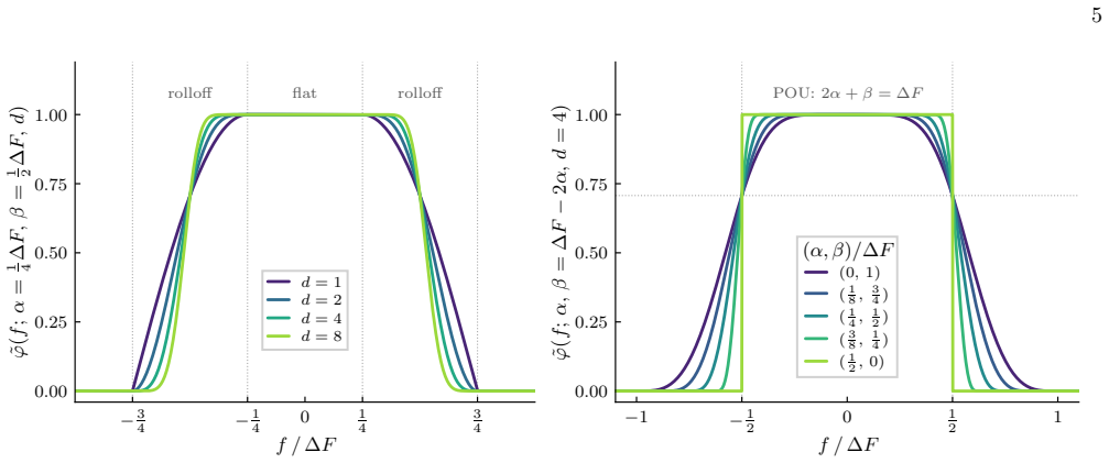
Normalization Forp=m,n=qthe inner product needs to normalize to unity. Momentarily restricting top=m̸= 0, N f, we find F + = Z +∞ −∞ ˜ϕ(x)˜ϕ(x+ 2m∆F) dx= 0,(B10) as ˜ϕ(x) and ˜ϕ(x+ 2m∆F) have no overlapping support, and F − = Z +∞ −∞ ˜ϕ(x)2 dx= 1 ∆F Z +∞ −∞ ˜φ(x)2 dx .(B11) The integral of the Meyer filter can be split off in the flat and rolloff regions:...
-
[19]
The inner product reduces to O= 2A 2 m(−1)(n−q)mℜ(C ∗ mnCmq)F − .(B20) •Case 1:n−qis odd
Orthogonality,p=m,n̸=q Settingp=m̸= 0, N f,n̸=qwe again get F + = Z +∞ −∞ e−2πi(n−q)x∆T ˜ϕ(x)˜ϕ(x+ 2m∆F) dx= 0,(B18) as the filters in the integrand share no support, and F − = Z +∞ −∞ e−2πi(n−q)x∆T ˜ϕ(x)2 dx .(B19) This expression amounts to the Fourier transform of ˜ϕ(x)2 and thusF − is real, as ˜ϕ(x)2 is real and even. The inner product reduces to O= 2...
-
[20]
Orthogonality,|p−m|= 1 We restrict to 1< p=m+ 1< N f without loss of generality, as them=p+ 1 case follows by symmetry. Now F + = Z +∞ −∞ e−2πi(n−q)x∆T ˜ϕ(x)˜ϕ(x+ (2m+ 1)∆F) dx= 0,(B30) as the filters have no support, and F − = Z +∞ −∞ e−2πi(n−q)x∆T ˜ϕ(x)˜ϕ(x+ ∆F) dx .(B31) The inner product reduces to O= 2A mAm+1(−1)(n−q)mℜ C ∗ mnC(m+1)qF − .(B32) The su...
-
[21]
Isolated neutron star signals are intrinsically compact in frequency
(F2) This sinc function is maximized atf= 0 and falls off as 1/fand therefore has infinite second frequency moment Z ∞ −∞ f2|˜gm(f)|2 df∼ Z ∞ −∞ df=∞.(F3) As an outcome, the transform of a signal has support beyond the time-frequency bins the signal crosses, smearing to adjacent frequencies as 1/f. Isolated neutron star signals are intrinsically compact i...
-
[22]
Gabor, Theory of communication, Journal of the Institution of Electrical Engineers93, 429 (1946)
D. Gabor, Theory of communication, Journal of the Institution of Electrical Engineers93, 429 (1946). 37
1946
-
[23]
Balian, Un principe d’incertitude fort en th’eorie du signal ou en m’ecanique quantique, Comptes Rendus de l’Acad’emie des Sciences de Paris, S’erie II292, 1357 (1981)
R. Balian, Un principe d’incertitude fort en th’eorie du signal ou en m’ecanique quantique, Comptes Rendus de l’Acad’emie des Sciences de Paris, S’erie II292, 1357 (1981)
1981
-
[24]
F. E. Low, Complete sets of wave packets, inA Passion for Physics—Essays in Honor of Geoffrey Chew(World Scientific,
-
[25]
S. Klimenko, S. Mohanty, M. Rakhmanov, and G. Mitselmakher, Constraint likelihood analysis for a network of gravita- tional wave detectors, Phys. Rev. D72, 122002 (2005), arXiv:gr-qc/0508068
Pith/arXiv arXiv 2005
-
[26]
K. G. Wilson, Generalized Wannier functions (1987), cornell University preprint
1987
-
[27]
Daubechies, S
I. Daubechies, S. Jaffard, and J.-L. Journ´ e, A simple wilson orthonormal basis with exponential decay, SIAM Journal on Mathematical Analysis22, 554 (1991)
1991
-
[28]
Meyer,Wavelets and Operators, Cambridge Studies in Advanced Mathematics, Vol
Y. Meyer,Wavelets and Operators, Cambridge Studies in Advanced Mathematics, Vol. 37 (Cambridge University Press, Cambridge, 1992)
1992
-
[29]
N. J. Cornish, Time-Frequency Analysis of Gravitational Wave Data, Phys. Rev. D102, 124038 (2020), arXiv:2009.00043 [gr-qc]
arXiv 2020
-
[30]
C. Cutler and E. E. Flanagan, Gravitational waves from merging compact binaries: How accurately can one extract the binary’s parameters from the inspiral wave form?, Phys. Rev. D49, 2658 (1994), arXiv:gr-qc/9402014
Pith/arXiv arXiv 1994
- [31]
-
[32]
Wiener, Generalized harmonic analysis, Acta Math.55, 117 (1930)
N. Wiener, Generalized harmonic analysis, Acta Math.55, 117 (1930)
1930
-
[33]
Khinchin, Korrelationstheorie der station¨ aren stochastischen Prozesse, Math
A. Khinchin, Korrelationstheorie der station¨ aren stochastischen Prozesse, Math. Ann.109, 604 (1934)
1934
-
[34]
Whittle, Curve and Periodogram Smoothing, J
P. Whittle, Curve and Periodogram Smoothing, J. Roy. Stat. Soc. B19, 38 (1957)
1957
-
[35]
Necula, S
V. Necula, S. Klimenko, and G. Mitselmakher, Transient analysis with fast wilson-daubechies time-frequency transform, Journal of Physics: Conference Series363, 012032 (2012)
2012
-
[36]
Colpiet al., LISA Definition Study Report, arXiv:2402.07571 [astro-ph.CO] (2024)
M. Colpiet al., LISA Definition Study Report, arXiv:2402.07571 [astro-ph.CO] (2024)
Pith/arXiv arXiv 2024
-
[37]
M. C. Digman and N. J. Cornish, LISA Gravitational Wave Sources in a Time-varying Galactic Stochastic Background, Astrophys. J.940, 10 (2022), arXiv:2206.14813 [astro-ph.IM]
arXiv 2022
-
[38]
M. C. Digman and N. J. Cornish, Parameter estimation for stellar-origin black hole mergers in LISA, Phys. Rev. D108, 023022 (2023), arXiv:2212.04600 [gr-qc]
arXiv 2023
-
[39]
Johnson, K
A. Johnson, K. Chatziioannou, and R. Rosati, The wdm time-frequency transform in gravitational-wave data analysis II: Evolutionary spectrum and noise covariance (2026), in preparation
2026
-
[40]
M. L. Katz, N. Karnesis, N. Korsakova, J. R. Gair, and N. Stergioulas, Efficient GPU-accelerated multisource global fit pipeline for LISA data analysis, Phys. Rev. D111, 024060 (2025), arXiv:2405.04690 [gr-qc]
arXiv 2025
-
[41]
LIGO Scientific Collaboration, Virgo Collaboration, and KAGRA Collaboration, LVK Algorithm Library - LALSuite, Free software (GPL) (2018)
2018
-
[42]
J. D. E. Creighton and W. G. Anderson,Gravitational-Wave Physics and Astronomy: An Introduction to Theory, Exper- iment and Data Analysis(Wiley, 2011)
2011
-
[43]
J. D. Markel, FFT pruning, IEEE Trans. Audio Electroacoust.19, 305 (1971)
1971
-
[44]
C. R. Harris, K. J. Millman, S. J. van der Walt, R. Gommers, P. Virtanen, D. Cournapeau, E. Wieser, J. Taylor, S. Berg, N. J. Smith, R. Kern, M. Picus, S. Hoyer, M. H. van Kerkwijk, M. Brett, A. Haldane, J. F. del R´ ıo, M. Wiebe, P. Peterson, P. G´ erard-Marchant, K. Sheppard, T. Reddy, W. Weckesser, H. Abbasi, C. Gohlke, and T. E. Oliphant, Array progra...
2020
-
[45]
N. J. Cornish, Non-stationary noise in gravitational wave analyses: The wavelet domain noise covariance matrix, arXiv:2511.10632 [gr-qc] (2025)
Pith/arXiv arXiv 2025
-
[46]
N. Pearson and N. J. Cornish, Handling data gaps for the next generation of gravitational-wave observatories, Phys. Rev. D113, 064033 (2026), arXiv:2509.05479 [gr-qc]
Pith/arXiv arXiv 2026
-
[47]
Virtanen, R
P. Virtanen, R. Gommers, T. E. Oliphant, M. Haberland, T. Reddy, D. Cournapeau, E. Burovski, P. Peterson, W. Weckesser, J. Bright, S. J. van der Walt, M. Brett, J. Wilson, K. J. Millman, N. Mayorov, A. R. J. Nelson, E. Jones, R. Kern, E. Larson, C. J. Carey, ˙I. Polat, Y. Feng, E. W. Moore, J. VanderPlas, D. Laxalde, J. Perktold, R. Cimrman, I. Henriksen,...
2020
-
[48]
J. D. Hunter, Matplotlib: A 2D graphics environment, Computing in Science & Engineering9, 90 (2007)
2007
-
[49]
P. Jaranowski, A. Krolak, and B. F. Schutz, Data analysis of gravitational - wave signals from spinning neutron stars. 1. The Signal and its detection, Phys. Rev. D58, 063001 (1998), arXiv:gr-qc/9804014
Pith/arXiv arXiv 1998
-
[50]
P. R. Williams and B. F. Schutz, An Efficient matched filtering algorithm for the detection of continuous gravitational wave signals, AIP Conf. Proc.523, 473 (2000), arXiv:gr-qc/9912029
Pith/arXiv arXiv 2000
-
[51]
R. Tenorio and D. Gerosa, Scalable data-analysis framework for long-duration gravitational waves from compact binaries using short Fourier transforms, Phys. Rev. D111, 104044 (2025), arXiv:2502.11823 [gr-qc]
arXiv 2025
-
[52]
M. Du, Z. Luo, and P. Xu, Enhancing Taiji’s parameter estimation under nonstationarity: A time-frequency domain framework for Galactic binaries and instrumental noises, Phys. Rev. D112, 083036 (2025), arXiv:2506.10599 [gr-qc]
arXiv 2025
discussion (0)
Sign in with ORCID, Apple, or X to comment. Anyone can read and Pith papers without signing in.