REVIEW 3 major objections 6 minor 49 references
Infinite horizon billiards: Transport at the border between Gauss and L\'evy universality classes
T0 review · 3 major / 6 minor · reviewed 2026-08-14 · deepseek-v4-flash
Pith's one-line read The paper claims that for infinite-horizon Lorentz gases the full two-dimensional particle density follows from the geometric inter-collision time distribution, without fitting.
desk verdict A serious analytical push on the infinite-horizon Lorentz gas that mostly lands: geometric CDFs plus a Lambert-scaled Lévy walk reproduce the 2D density without fitting, though an arbitrary split constant and the stadium-channel effective fit keep it short of airtight. read the letter →
The pith
A machine-rendered reading of the paper's core claim, the machinery that carries it, and where it could break.
The reading
What carries the argument
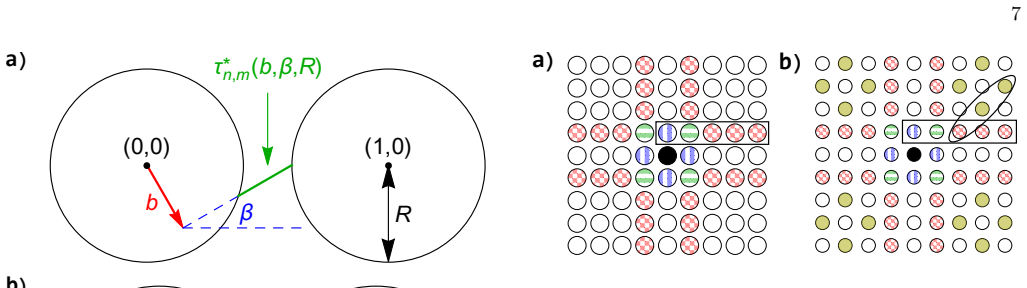
The central object is the inter-collision time distribution $\psi(\tau)$, computed as a sum over all reachable scatterers of integrals over the collision impact parameter $b$ and recoil angle $\beta$, with integration boundaries fixed by no-blocking conditions. Its tail $\psi(\tau)\sim \tau_0^2/\tau^3$ places the model at the border between Gaussian and Lévy statistics; Lambert scaling via the secondary branch $W_{-1}$ absorbs the logarithmically growing scale $\Omega_d(t)$ so finite-time results can be compared with theory. A discrete velocity distribution $F_2(\mathbf{v})$ with diagonal weight $q$ converts the geometry into the Lévy-walk (Montroll-Weiss) propagator.
What would settle it
A direct test: compute the particle density for the Lorentz gas at other scatterer radii within the two-corridor and four-corridor regimes, for example $R=0.35$ or $R=0.28$, and compare with Eq. (26) using only the geometry-derived constants; a mismatch in the corridor plume tails would show that the parameter-free reproduction is specific to the two sampled radii. A second check is a correlation plot of consecutive inter-collision times for $\tau$ values above the plateau region, where the paper's renewal diagnosis is read directly from the scatter.
Extended reading notes
Core claim
The central claim is that the geometry of an infinite-horizon Lorentz gas determines its finite-time transport statistics: the inter-collision time distribution $\psi(\tau)$ computed from the scatterer layout, combined with a discrete corridor velocity distribution and Lambert scaling, yields the full two-dimensional position density $P_2(\mathbf{r},t)$ that matches simulation 'without any fitting' for $R=0.3$ and $R=0.4$. The power-law corridor tails are part of this density, not a separate asymptotic correction, while the rigorous Gaussian limit exists only after an astronomically large number of collisions. For the stadium channel the paper claims a weaker statement: the Lévy-walk formula can still describe the density if effective waiting-time parameters are fitted, even though the renewal assumption itself fails there.
Load-bearing premise
The load-bearing premise is the renewal step: after each collision the next flight duration is drawn independently from the geometry-derived distribution, so deterministic correlations between flights can be dropped; the stadium-channel results show this premise is model-dependent and can fail.
Editorial extensions
If this is right
- For the infinite-horizon Lorentz gas, finite-time transport is describable by a Lévy walk with geometry-derived $\psi(\tau)$, and the Gaussian propagator is not observable on practical timescales.
- The Lambert-scaled formula supplies explicit finite-time corrections, including Kummer function terms, so simulations at times like $t=10^4$ can be compared with theory instead of waiting for $\sqrt{N\ln N}$ convergence.
- The packet's shape—cross-like for two corridors, British-flag-like for four—is encoded in the velocity distribution $F_2(\mathbf{v})$ and the parameter $q$ that measures diagonal corridor weight.
- For the stadium channel, an effective-parameter Lévy walk reproduces the density after fitting two constants even when the renewal assumption is invalid.
- The non-analytic, plateau-rich structure of the inter-collision time CDF reflects the periodic scatterer array and is inherited by the spreading density.
Reading between the lines
- If the parameter-free match persists at other scatterer radii, the same geometry-to-CDF recipe should transfer to other periodic lattices, where corridor directions and blocking conditions change but the $\tau^{-3}$ tail index suggests a common universality class.
- The paper's correlation plots of consecutive inter-collision times could be turned into a quantitative diagnostic: a measure of dependence in $(\tau_n,\tau_{n+1})$ would predict in advance which billiards admit a renewal description.
- The Lambert split parameter $\eta$ is the one empirical element in an otherwise derived chain; matching higher-order terms in the asymptotic expansion could fix it and remove the remaining freedom.
Signed reviews
Editorial analysis
A structured set of objections, weighed in public.
Referee Report
Summary. This paper studies finite-time transport in two deterministic billiard models with infinite horizons: the Lorentz gas on a square lattice with circular scatterers (two or four open corridors) and the stadium channel. The authors derive, from geometry and the assumption of uniform collision parameters, the cumulative distribution function of inter-collision times for each model (Eqs. (28), (33)-(47), (49), (55)-(58)), and the CDFs match single-trajectory simulations. They then model the spatial spreading with a Lévy walk whose velocity distribution is discrete (Eqs. (19), (24)), using a Lambert-W scaling to handle the logarithmic divergence at the border between Gaussian and Lévy statistics. The main claim is that for the Lorentz gas the position PDF (Eq. (26)) reproduces simulations without fitting, with constants τ0, ⟨τ⟩, Cψ, and q computed from the analytic ψ(τ), while for the stadium channel Eq. (23) describes the data only with two effective fitted parameters because the renewal assumption fails.
Significance. If the parameter-free claim held in full, the paper would provide a practically relevant mesoscopic propagator for the infinite-horizon Lorentz gas, bridging the regime where Bleher's Gaussian limit is not yet valid, and would explain the cross-like and British-flag shapes and the power-law corridor tails. The paper has real strengths: the geometric CDF formulas are tested against numerical histograms; the Lambert scaling is a useful resummation of the slow logarithmic factors; the correlation plots in Fig. 12 provide a direct diagnostic of the renewal assumption; and the authors are explicit that the stadium-channel case requires effective parameters and that renewal fails there. The main caveat is that the 'without any fitting' claim for the Lorentz gas is qualified by an unconstrained Lambert split parameter η and by the modeling ansatz for the velocity distribution.
major comments (3)
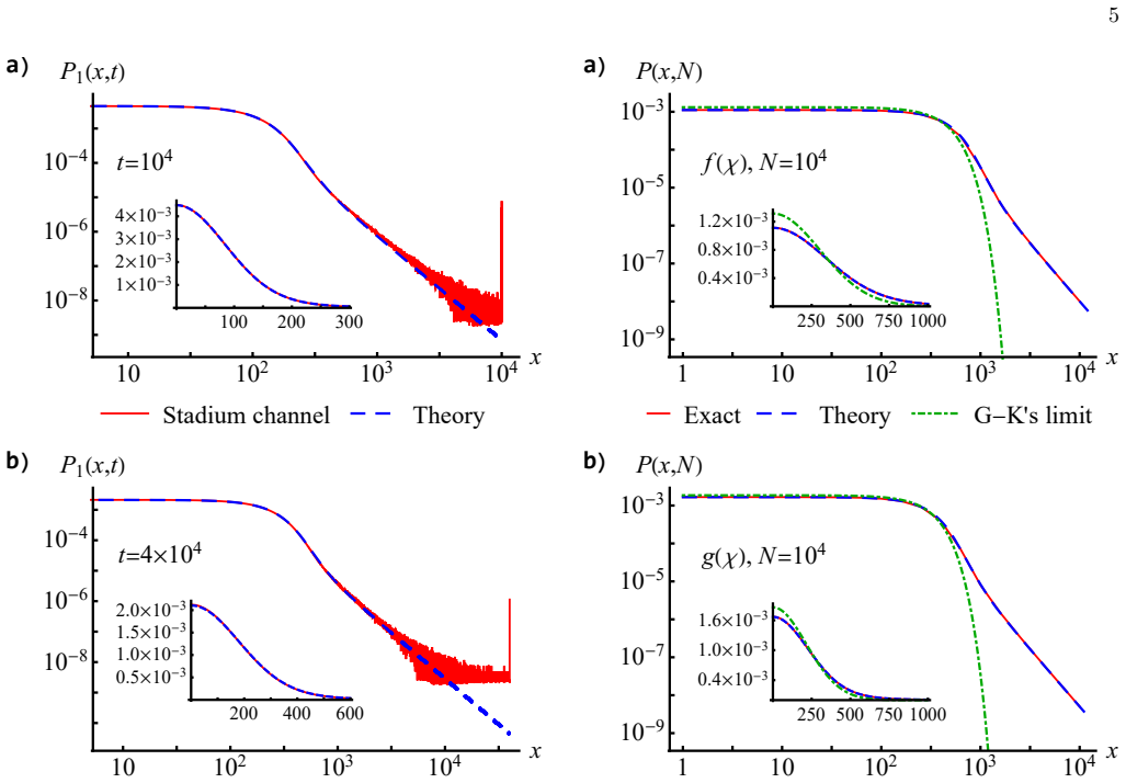
- [Section V, Eq. (60)] The Lambert split parameter η introduced in Eq. (60) is a free parameter, and the paper chooses η=1 because it 'produces good results' rather than from a dynamical or asymptotic condition. This is load-bearing because the O(1/Ω) term in Eqs. (10), (23), and (25), namely the Kummer correction, is precisely the term that produces the non-Gaussian tails emphasized in the paper. For the R=0.3 Lorentz gas and t=10^4, Eq. (21) gives Ω(t)≈8.2, so replacing η by eη changes the subleading term by roughly 12%; this is the same order as the difference between the theory and Bleher's Gaussian shown in Figs. 9 and 10. Consequently, the statement that Figs. 2, 3, 9, and 10 reproduce the simulation 'without any fitting' is not literally supported. Please either derive η from the asymptotic expansion, demonstrate insensitivity of the conclusions to η, or explicitly reclassify η as an empirically fixed resummation constant.
- [Section III, Eq. (24)] The velocity distribution F_2(v) used for the Lorentz gas is an effective ansatz rather than a consequence of the collision dynamics: the actual post-collision velocity is continuous and correlated with the incoming flight, while Eq. (24) replaces it by an IID draw restricted to the corridor directions, with the diagonal weight q taken from Eq. (47). The excellent agreement with particle simulations provides empirical support, but the paper does not test how much of the match depends on this particular ansatz, nor why the continuous components should be irrelevant. Because this choice is part of the claimed parameter-free mapping to the Lévy walk, the text should state explicitly that Eq. (24) is an effective distribution and should include at least one robustness check, such as an alternative q or a velocity distribution with continuous angular support.
- [Section V / Figs. 2, 3, 9, 10] The central claim of parameter-free reproduction of the Lorentz-gas density is supported only by visual log-density maps and two cross-sections. Since the claim is quantitative and the η ambiguity affects exactly the displayed non-Gaussian correction, the paper needs a quantitative comparison metric, such as relative L1 error or residual plots as a function of r at fixed t, to substantiate 'reproduces well' and 'without any fitting'. This is particularly important because the two cross-sections shown are along symmetry directions, while the full 2D comparison in Figs. 2 and 3 is only qualitative.
minor comments (6)
- [Section II/III headings] The headings 'LAMBER T SCALING' and 'LÉVY W ALK' contain spacing errors; they should read 'Lambert scaling' and 'Lévy walk'.
- [Section V] The text uses 'Lorenz gas' in the discussion of correlation patterns; this should be 'Lorentz gas'.
- [Section IV A] The condition for four open horizons is stated as '√20≤ R < 1/√8'; from the context and the later use of 1/√20, this should be 1/√20 ≤ R < 1/√8.
- [Reference [17]] Reference [17] has a typographical error: 'H. K. ZhangCommun. Math. Phys.' should read 'H. K. Zhang, Commun. Math. Phys.'
- [Section IV B] The uniformity of a and α in Eq. (49) is assumed rather than derived; the excellent CDF match in Fig. 11 supports the assumption, but a brief justification or citation would strengthen the presentation.
- [Section V / Fig. 4] The statement that Eq. (23) 'can indeed describe the stadium channel model' is stronger than the evidence, since the constants in Fig. 4 are obtained by a two-parameter fit; 'can be fitted to' or 'can effectively describe' would be more accurate.
Circularity Check
No significant circularity: the Lorentz-gas density prediction is produced from first-principles geometric collision-time distributions and checked against independent simulations, with the only free convention (eta=1) disclosed and fixed in a separate IID test.
full rationale
The central Lorentz-gas claim is not circular. The constants tau_0, <tau>, and C_psi inserted into the Levy-walk expression Eq. (26) are computed from the geometric CDF of inter-collision times, Eqs. (28)-(46), and then compared with particle simulations in Figs. 2, 3, 9, and 10. The four-corridor weight q is defined in Eq. (47) as the ratio of the diagonal-corridor contribution to the total tau_0^2 obtained from the same geometric CDF, not fitted to the density. The stadium-channel section is explicit that the effective constants come from a two-parameter fit at t=10^4 and are then used for t=4x10^4, so this is disclosed fitting rather than a fitted input disguised as a prediction. The Lambert split eta is acknowledged in Section V as a free parameter that cannot be fixed by the derivation; it is chosen once in the IID toy model and validated there against the exact inverse Fourier transform (Fig. 5), then carried into the billiard model without adjustment to the billiard data. This is a sensitivity/correctness concern, not circularity. Self-citation [23] is used only as a cross-check of tau_0 that is independently re-derived here, so it is not load-bearing. The paper also explicitly reports where the renewal assumption fails (stadium channel), further indicating that the successful Lorentz-gas case is not manufactured by construction.
Assumptions & free parameters
free parameters (3)
- Lambert split parameter eta =
1
- Stadium effective C_psi^2 <tau> =
0.3776
- Stadium effective <tau> / tau0^2 =
7.0607
assumptions (5)
- domain assumption Collision parameters (impact parameter and recoil angle) are uniformly distributed: b and beta for the Lorentz gas, a and alpha for the stadium channel.
- domain assumption Renewal assumption: flight times and velocities in the Lévy walk are IID, so the Montroll-Weiss equation (14) applies.
- domain assumption Small-u and small-k scaling ansatz u ~ k^2 L(k) with u << k, used to expand the Montroll-Weiss equation.
- ad hoc to paper Effective velocity distribution F_2(v) in Eq. (24) is confined to corridor directions, with diagonal weight q from Eq. (47).
- domain assumption Finite mean inter-collision time and finite velocity moments.
Cite this review
Pith. "Pith review of Infinite horizon billiards: Transport at the border between Gauss and L\'evy universality classes." pith.science (2026). https://pith.science/paper/HU3SF7EN
@misc{pith2026190802053,
  author       = {Pith},
  title        = {Pith review of: Infinite horizon billiards: Transport at the border between Gauss and L\'evy universality classes},
  year         = {2026},
  howpublished = {\url{https://pith.science/paper/HU3SF7EN}},
  note         = {Machine review of arXiv:1908.02053}
}
read the original abstract
We consider transport in two billiard models, the infinite horizon Lorentz gas and the stadium channel, presenting analytical results for the spreading packet of particles. We first obtain the cumulative distribution function of traveling times between collisions, which exhibits non-analytical behavior. Using a renewal assumption and the L\'evy walk model, we obtain the particles' probability density. For the Lorentz gas, it shows a distinguished difference when compared with the known Gaussian propagator, as the latter is valid only for extremely long times. In particular, we show plumes of particles spreading along the infinite corridors, creating power-law tails of the density. We demonstrate the slow convergence rate via summation of independent identically distributed random variables on the border between L\'evy and Gauss laws. The renewal assumption works well for the Lorentz gas with intermediately sized scattering centers, but fails for the stadium channel due to strong temporal correlations. Our analytical results are supported with numerical samplings.
Figures


Figures from the paper (9 more)



Reference graph
Works this paper leans on
-
[1]
In order to find the leading behavior of the second term of Eq
A non-integer ν Let us assume that¯n−1<ν < ¯n. In order to find the leading behavior of the second term of Eq. (A4), we consider the limit l0 = lim k→0+ 1 kν ∫ ∞ −∞ dχf (χ) [ eikχ− ¯n−1∑ n=0 (ikχ)n n! ] . (A5) 15 Using L’Hospital’s rule¯n times yields l0 = lim k→0+ Γ(−ν)(−i)¯n Γ(−ν + ¯n) k¯n−ν ∫ ∞ −∞ dχf (χ)χ¯neikχ, (A6) where Γ(··· ) is the Gamma function...
-
[2]
In order to find the leading behavior of the second term of Eq
An integer ν Let us assume thatν = ¯n, where ¯n is even. In order to find the leading behavior of the second term of Eq. (A4), we consider the limit l1 = lim k→0+ 1 k¯n ln(k) ∫ ∞ −∞ dχf (χ) [ eikχ− ¯n−1∑ n=0 (ikχ)n n! ] . (A9) Using L’Hospital’s rule¯n + 1 times produces l1 = i¯n+1 ¯n! lim k→0+ k ∫ ∞ −∞ dχf (χ)χ¯n+1eikχ. (A10) Changing the integration vari...
-
[3]
M. Courbage, M. Edelman, S. M. Saberi Fathi, and G. 25 M. Zaslavsky,Phys. Rev. E 77, 036203 (2008)
work page 2008
-
[4]
(D7) The separator angle between (I) and (II) can be found by comparing the lower (or upper)b IB of (i) to that of (ii), yielding β = cos−1(2R). Therefore we find forn = 1 (I) π 4− sin−1 (√ 2R ) ≤β≤ cos−1(2R), (i) cos(β)− sin(β)−R≤b≤R, (D8) and (II) cos−1(2R)≤β≤ π 4, (ii) R− sin(β)≤b≤ cos(β)−R. (D9) Finally, Eq. (32) in its explicit form supply (i) cos(β)−...
-
[5]
(A8), and take the limit ofν→ ¯n, where ¯n is odd
(A12) If ¯n is odd, we return to Eq. (A8), and take the limit ofν→ ¯n, where ¯n is odd. We obtain l1 = lim ν→¯n 2χν 0Γ(−ν) cos (πν 2 ) = π ¯n!(−1) ¯n+1 2 χ¯n
-
[6]
(A13) To compute the next order correction for the case of an even¯n, we calculate the following limit l2 = lim k→0+ 1 k¯n {∫ ∞ −∞ dχf (χ) [ eikχ− ¯n−1∑ n=0 (ikχ)n n! ] + 2 ¯n!(−1)¯n/2(χ0k)¯n ln(k) } . (A14) Using L’Hospital’s rule¯n times results with l2 = (−1)¯n/2 ¯n! lim k→0+ {∫ ∞ −∞ dχf (χ)χ¯neikχ + 2χ¯n 0 [ ln(k) +H¯n ]} , (A15) where H¯n =∑¯n n=1 1 ...
-
[7]
In order to obtain the leading behavior of the second term of Eq
A non-integer ν Let us assume that ˜n− 1 < ν <˜n. In order to obtain the leading behavior of the second term of Eq. (B4), we consider the limit l0 = lim u→0 1 uν ∫ ∞ 0 dτψ (τ) [ e−uτ− ¯n−1∑ n=0 (−uτ)n n! ] . (B5) 17 Using L’Hospital’s rule˜n times yields l0 = lim u→0 Γ(−ν)u¯n−ν Γ(−ν + ¯n) ∫ ∞ 0 dτψ (τ)τ ¯ne−uτ. (B6) Changing the integration variable toη =...
-
[8]
We also get fromψ(τ) numer- ical values for⟨τ⟩ andCψ for this specific value ofR, see appendix E. We find that⟨τ⟩≈ 1.1947, with a relative error of 0.059% to the rigorous result Eq. (38), and also Cψ≈ 1.5250× 10⁻². These values provide excellent re- sults for the numerical simulations of the position’s PDF when used as an input for the Lévy walk approximati...
work page 1947
Show all 49 references
-
[9]
In order to find the leading behavior of Eq
An integer ν Let us assume thatν = ¯n, where ¯n can be even or odd. In order to find the leading behavior of Eq. (B4), we consider the following limit l1 = lim u→0 1 u¯n ln(u) ∫ ∞ 0 dτψ (τ) [ e−uτ− ¯n−1∑ n=0 (−uτ)n n! ] . (B9) Using L’Hospital’s rule˜n + 1, we get l1 = lim u→0 ...
-
[10]
(B13) We use L’Hospital’s rule¯n times to get l2 = (−1)¯n ¯n! lim u→0 {∫ ∞ 0 dτψ (τ)τ ¯ne−uτ +τ ¯n 0 [ ln(u) +H¯n ]} , (B14) where H¯n =∑¯n n=1 1 n is the ¯nth harmonic number
(B12) To obtain the next order correction, we evaluate the following limit l2 = lim u→0 1 u¯n {∫ ∞ 0 ψ(τ) [ e−uτ− ¯n−1∑ n=0 (−uτ)n n! ] dτ− τ ¯n 0 ¯n! (−1)¯n+1u¯n ln(u) } . (B13) We use L’Hospital’s rule¯n times to get l2 = (−1)¯n ¯n! lim u→0 {∫ ∞ 0 dτψ (τ)τ ¯ne−uτ +τ ¯n 0 [ l...
-
[11]
The pair{b,β} and the trio{x0,y 0,β} are related by a simple transformation
Lorentz gas model We denote as(x0,y 0) the starting point on the(0, 0) scatterer from which we assume the particle has originated. The pair{b,β} and the trio{x0,y 0,β} are related by a simple transformation. To obtain it, we define the two vectors R =x0ˆx +y0ˆy, B =−b sin(β)ˆx ...
-
[12]
The pair{a,α} and the trio{x0,y 0,α} are related by a simple transformation
Stadium channel model We denote as(x0,y 0) the starting point on the(0, 0) stadium from which we assume the particle has originated. The pair{a,α} and the trio{x0,y 0,α} are related by a simple transformation. To obtain it, we define the two vectors R =x0ˆx +y0ˆy, A =−a sin(α)ˆ...
-
[13]
(28) together with the integration boundaries Eqs
Lorentz gas model Using Eq. (28) together with the integration boundaries Eqs. (33-36), one can calculateψ(τ) using a computational program like Mathematica and extract the constantsτ0,⟨τ⟩, andCψ out of it. However, we found that an analytical expression forτ0 can be calculate...
-
[14]
(28) into Eq
Plugging Eq. (28) into Eq. (E1) gives τ 2 0 = 2 πR (1− 2R)2 + 8 lim T→∞ 1 T ∞∑ m=1 ∫ βmax m+1,m(R) βmin m+1,m(R) dβ 2π ∫ bmax m+1,m(β,R) bmin m+1,m(β,R) db 2Rτ∗3 m+1,m(b,β,R )H [ T−τ∗ m+1,m(b,β,R ) ] . (E12) Using geometrical considerations, this time we haveτ∗ m+1,m(b,β,R )≃ ...
1947
-
[15]
Sinceτ∗ 2n,D(a,α ) is the traveling distance to thenth upper semicircle, it is clear thatτ∗ 2n,D(a,α )≃ √ (2n + 2)2 +D2 when n is large
Stadium channel model We use an identical way as for the Lorentz gas to computeτ0 analytically. Sinceτ∗ 2n,D(a,α ) is the traveling distance to thenth upper semicircle, it is clear thatτ∗ 2n,D(a,α )≃ √ (2n + 2)2 +D2 when n is large. Plugging Eq. (49) into Eq. (E1) and employin...
-
[16]
H. A. Lorentz,KNA W Proceedings7, 438 (1905)
1905
-
[17]
J. P. Bouchaud and P. Le Doussal,J. Stat. Phys. 41, 225 (1985)
1985
-
[18]
D. I. Dolgopyat and N. L. Chernov,Russ. Math. Surv. 64, 651 (2009)
2009
-
[19]
Cristadoro, T
G. Cristadoro, T. Gilbert, M. Lenci, and D. P. Sanders, Phys. Rev. E 90, 050102(R) (2014)
2014
-
[20]
Cristadoro, T
G. Cristadoro, T. Gilbert, M. Lenci, and D. P. Sanders, Phys. Rev. E 90, 022106 (2014)
2014
-
[21]
M.Feliczaki, E.Vicentini, andP.P.González-Borrero, Phys
R. M.Feliczaki, E.Vicentini, andP.P.González-Borrero, Phys. Rev. E 96, 052117 (2017)
2017
-
[22]
Klages, S
R. Klages, S. S. G. Gallegos, J. Solanpää, M. Sarvilahti, and E. Räsänen,Phys. Rev. Lett. 122, 064102 (2019)
2019
-
[23]
Vollmer, L
J. Vollmer, L. Rondoni, M. Tayyab, C. Giberti, and C. Mejía-Monasterio, arXiv:1903.12500 [cond-mat.stat- mech]
1903 arXiv
-
[24]
L. A. Bunimovich,Commun. Math. Phys. 65, 295 (1979)
1979
-
[25]
Boldrighini, L
C. Boldrighini, L. A. Bunimovich, and Y. G. Sinai,J. Stat. Phys. 32, 477 (1983)
1983
-
[26]
L. A. Bunimovich,Zh. Eksp. Teor. Fiz. 89, 1452 (1985)
1985
-
[27]
P. M. Bleher,J. Stat. Phys. 66, 315 (1992)
1992
-
[28]
Dahlqvist,Nonlinearity 10, 159 (1997)
P. Dahlqvist,Nonlinearity 10, 159 (1997)
1997
-
[29]
Szász and T
D. Szász and T. Varjú,J. Stat. Phys. 129, 59 (2007)
2007
-
[30]
F.P.BocaandA.Zaharescu, Commun. Math. Phys. 269, 425 (2007)
2007
-
[31]
Chernov,J
N. Chernov,J. Stat. Phys. 127, 1 (2007)
2007
-
[32]
gallery whis- pering paths
could probably supply one with tools to approximate edge phenomena such as this. Finally, we address the reader to interesting corre- lation patterns of the stadium channel model, seen in Fig. 12 (b). We plot points of consecutive traveling times (τn+1,τn), for the Lorentz gas...
-
[33]
Chernov and H
N. Chernov and H. K. ZhangCommun. Math. Phys. 277, 305 (2008)
2008
-
[34]
Marklof and A
J. Marklof and A. Strömbergsson, Geom. Funct. Anal. 21, 560 (2011)
2011
-
[35]
C. P. Dettmann,J. Stat. Phys. 146, 181 (2012)
2012
-
[36]
C. P. Dettmann,Commun. Theor. Phys. 62, 521 (2014)
2014
-
[37]
Marklof and B
J. Marklof and B. Tóth,Commun. Math. Phys. 347, 933 (2016)
2016
-
[38]
Zarfaty, A
L. Zarfaty, A. Peletskyi, I. Fouxon, S. Denisov, and E. Barkai, Phys. Rev. E 98, 010101(R) (2018)
2018
-
[39]
M. F. Shlesinger, B. J. West, and J. Klafter,Phys. Rev. Lett. 58, 1100 (1987)
1987
-
[40]
Zaburdaev, S
V. Zaburdaev, S. Denisov, and J. Klafter, Rev. Mod. Phys. 87, 483 (2015)
2015
-
[41]
Zaburdaev, I
V. Zaburdaev, I. Fouxon, S. Denisov, and E. Barkai, Phys. Rev. Lett. 117, 270601 (2016)
2016
-
[42]
Fouxon, S
I. Fouxon, S. Denisov, V. Zaburdaev, and E. Barkai,J. Phys. A 50, 154002 (2017)
2017
-
[43]
Börgersa and C
C. Börgersa and C. Greengard,Comptes Rendus Mathe- matique 356, 6 (2018)
2018
-
[44]
Refer to http://functions.wolfram.com for more informa- tion
-
[45]
Gnedenko and A.N
B.V. Gnedenko and A.N. Kolmogorov, Limit distribu- tions for sums of independent random variables , Addison- Wesley, Cambridge (1968)
1968
-
[46]
E. W. Montroll and G. H. Weiss,J. Math. Phys. 6, 167 (1965)
1965
-
[47]
Rebenshtok, S
A. Rebenshtok, S. Denisov, P. Hänggi, and E. Barkai, Phys. Rev. Lett. 112, 110601 (2014)
2014
- [48]
-
[49]
C. M. Bender and S. A. Orszag,Advanced mathematical methods for scientists and engineers , McGraw-Hill, New York (1978)
1978
Reviewed August 14, 2026 · model on record in the stance chip above.
Discussion (0). Continue with ORCID to comment.