REVIEW 4 major objections 6 minor 34 references
Transition to Turbulence in Driven Active Matter
T0 review · 4 major / 6 minor · reviewed 2026-08-14 · deepseek-v4-flash
Pith's one-line read A driven active matter model reaches turbulence through a complete period-doubling cascade.
desk verdict A Lorenz-like active-matter model shows a novel period-halving/doubling route to chaos, but the 'complete cascade' and 'physical relevance' claims outrun the evidence. read the letter →
The pith
A machine-rendered reading of the paper's core claim, the machinery that carries it, and where it could break.
The reading
What carries the argument
The load-bearing object is the three-mode Galerkin truncation of the active-matter partial differential equations, obtained by keeping one roll velocity mode and two concentration modes: $\dot{X}=\sigma(-X+rY+rYZ)$, $\dot{Y}=-XZ+X-Y$, $\dot{Z}=-2Z+XY$. Here $X,Y$ describe the convective roll amplitudes, $Z$ the active-particle transport, $\sigma=\nu/D$ is the inverse Schmidt number, and $r=N/N_c$ is the control parameter; the term $rYZ$ in the first equation is the active-matter contribution that separates the model from the standard Lorenz system. The paper supplements the ODE with a Krylov-Bogolyubov amplitude expansion giving $[4\sigma-2i\omega_H\sigma] dA/dt = 8\sigma(\Delta r)A - 4A^3\sigma + O(1/\sigma)$, which shows the Hopf bifurcation is forward for large $\sigma$ and backward for small $\sigma$. Numerical solution of the ODE fixes the homoclinic locus $r_0(\sigma)$ and the Hopf locus $r_H(\sigma)$, which together locate the period-halving and period-doubling region and the coexistence window.
What would settle it
Directly simulate the full PDEs, Eqs. (2.1)-(2.3), at $\sigma=30$ with stress-free plates and a fixed concentration gradient, and increase $r$ through $r_H$: if the first oscillatory state is not a high-period limit cycle that halves to the $2\pi/\omega_H$ cycle and then period-doubles to a strange attractor, the paper's central claim fails. An experiment on a dense bacterial suspension that measures the vertical concentration flux while the imposed gradient is ramped would provide the same test.
Extended reading notes
Core claim
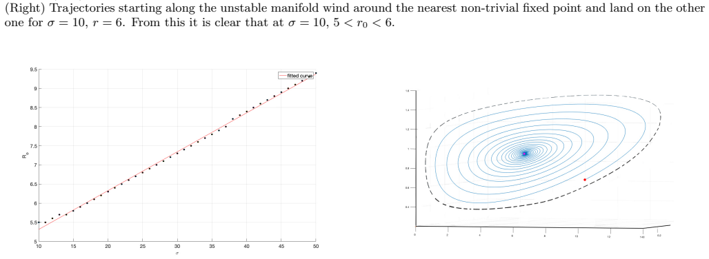
The central claim is that the driven active-matter Lorenz model, whose first equation contains the active-matter nonlinearity $rYZ$, has a Hopf bifurcation that is forward for large inverse Schmidt number $\sigma$ and backward for small $\sigma$, with the crossover near $\sigma\approx 21$. For $\sigma>21$, increasing the activity Rayleigh number $r=N/N_c$ past the Hopf point $r_H$ produces a stable high-period limit cycle of period $64\,(2\pi/\omega_H)$; this cycle period-halves down to a $2\pi/\omega_H$ cycle and then period-doubles into a Lorenz-like strange attractor. Below $\sigma\approx 21$, the system instead behaves like the standard Lorenz model: a homoclinic bifurcation at $r_0<r_H$ creates an unstable limit cycle, and chaos appears through the usual Lorenz mechanism without any period-doubling cascade. The paper also finds that for high $\sigma$ in the window $r_0<r<r_H$, a strange attractor coexists with stable nontrivial fixed points. The authors state this is the first time a Lorenz-like model has shown consecutive period-doubling bifurcations in a physically relevant transition to turbulence.
Load-bearing premise
The three-mode Galerkin truncation in Eqs. (2.16a)-(2.16c) captures the true dynamics of the full active-matter partial differential equations, so the period-doubling sequence in the ODE really is how the fluid becomes turbulent.
Editorial extensions
If this is right
- For $\sigma>21$, the route from the motionless state to chaos is: trivial state, two stable convective fixed points, Hopf birth of a high-period limit cycle, period-halving to a $2\pi/\omega_H$ cycle, then a sequence of period-doubling bifurcations to a strange attractor.
- The Hopf bifurcation is supercritical for large $\sigma$, with the limit-cycle amplitude growing as $\sqrt{\Delta r}$, unlike the subcritical Hopf bifurcation of the standard Lorenz model at comparable parameters.
- In the high-$\sigma$ window $r_0<r<r_H$, the strange attractor and stable fixed points coexist, so the final state depends on initial conditions and the transition is hysteretic.
- In the $\sigma\to\infty$ limit the first equation slaves $X$ to $Y$ and $Z$, leaving a two-dimensional flow, so chaos and the cascade disappear at extreme $\sigma$; the regime above $\sigma\approx21$ is therefore the physically relevant one.
- For $\sigma<21$ the model reproduces the standard Lorenz behavior of homoclinic chaos with no period-doubling cascade.
Reading between the lines
- The ODE analysis does not by itself prove that the Galerkin truncation survives contact with the full PDEs; the Ginzburg-Landau-type terms and higher-gradient nonlinearities dropped in Sec. II could move $r_H$ or destabilize the cascade, and a direct numerical simulation of Eqs. (2.1)-(2.3) is the natural check.
- Because the extra nonlinearity $rYZ$ is what makes the first equation depart from Lorenz, the same mechanism may produce complete cascades in other Lorenz-like models whose first equation couples the two passive modes, suggesting a broader class of all-nonlinear Lorenz systems.
- An experimental signature of the paper's scenario is a high-period oscillatory convective state just above onset, followed by period-halving and then period-doubling as the imposed gradient is increased; measuring the oscillation period and counting those steps would test the model without resolving individual swimmer trajectories.
- The predicted coexistence of a strange attractor with stable convection implies that the active-particle flux across the cell should show hysteresis when the imposed gradient is swept up and then down, a macroscopic observable test.
Signed reviews
Editorial analysis
A structured set of objections, weighed in public.
Referee Report
Summary. The paper studies a three-mode Lorenz-like ODE model for driven active matter, with nonlinear terms in all three equations. The model is derived from a simplified active-fluid PDE system (Eqs. 2.1-2.3) by a Galerkin truncation. The authors analyze the fixed points, the Hopf bifurcation, and a homoclinic orbit, and present numerical evidence of a route to chaos: for inverse Schmidt numbers σ above a critical value near 21, the trivial state, steady convection, a high-period limit cycle, a period-halving sequence to a T-period cycle, and then a sequence of period-doubling bifurcations to a strange attractor. The paper claims that this is the first observation of consecutive period-doubling bifurcations in a physically motivated Lorenz-like model.
Significance. If the claims are correct, the paper provides a low-dimensional example of a Feigenbaum-like route to turbulence in a hydrodynamic active-matter context, and it includes an analytic amplitude-equation derivation (Appendix A) for the Hopf bifurcation. The distinction from the standard Lorenz model—an extra nonlinear term in the X-equation—is clear and physically motivated. However, the central physical claim depends on an unvalidated three-mode truncation, and the connection between the analytic Hopf analysis and the numerically observed high-period orbit is not established. The paper also lacks quantitative diagnostics typical for period-doubling cascades (e.g., Feigenbaum ratios, Lyapunov exponents). These gaps prevent the manuscript from being accepted in its current form.
major comments (4)
- [II, Eqs. (2.1)-(2.3), (2.16)-(2.17)] The physical claim that this model describes a transition to turbulence in driven active matter rests on the three-mode Galerkin truncation of Eqs. (2.16a)-(2.16c), but the manuscript provides no evidence that the omitted terms and modes preserve the bifurcation structure. The text explicitly states (Sec. II) that the Ginzburg-Landau-like terms of Ref. [18] and a higher-gradient nonlinearity in the concentration current have been dropped, and no check against the full PDEs (2.1)-(2.3), no higher-mode truncation, and no experimental comparison is performed. Since the reported period-doubling cascade could be an artifact of the truncation, this missing validation is load-bearing for the central claim.
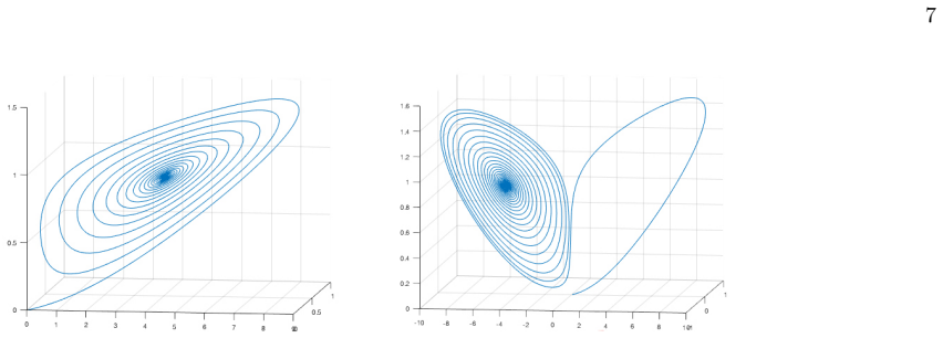
- [III and IV, Eq. (A.18), Fig. 11] There is a disconnect between the analytical Hopf bifurcation analysis and the numerical route to chaos. The amplitude equation (A.18) describes a supercritical Hopf bifurcation and therefore predicts a small-amplitude limit cycle with period approximately 2π/ω_H near r_H. However, Fig. 11a shows a stable limit cycle just above r_H with period 64(2π/ω_H) (the text reports T=8.94 at σ=30). The paper does not explain how the forward Hopf bifurcation yields a period-64 orbit, and the sequence from the high-period cycle to the T-period cycle (period-halving) is not derived analytically. The analytic and numeric pictures are therefore not connected.
- [Eq. (3.10) vs Eq. (A.11)] The scaling of the Hopf frequency is inconsistent between the main text and the appendix. For σ≫1, r_H≈σ/4, so Eq. (3.10) gives ω_H^2=8σ(r_H−1)≈2σ^2. In contrast, Eq. (A.11) states ω_H^2≈2σ. This discrepancy affects the large-σ scalings used in the derivation of the amplitude equation (A.18), because terms such as σ^2+9ω^2 and the factor (4σ−2iω_Hσ) are evaluated with different assumptions about ω_H. The claimed supercriticality of the Hopf bifurcation is therefore not reliably established.
- [IV, Fig. 11 and abstract] The claim of a 'complete' sequence of period-doubling bifurcations is not substantiated by quantitative diagnostics. The paper shows phase portraits at selected r values but does not compute Lyapunov exponents, locate the period-doubling bifurcation points, or estimate the Feigenbaum ratio. In addition, the period-halving sequence in Fig. 11a-e is not a successive halving (64→8→4→2→1 includes a factor-8 step), and the periods of the orbits in Fig. 11g-j are not labeled. Without these quantitative checks, 'complete' is an overstatement.
minor comments (6)
- [III, Eq. (3.2a)] The expression for X0 contains an inner ± sign; the minus branch yields no real solution for r>1, so the existence of just two nontrivial fixed points should be stated more clearly.
- [IV, Sec. II] The statement that σ=ν/D is the 'inverse Schmidt number' is inconsistent with the standard definition (Schmidt number Sc=ν/D). Please clarify the terminology.
- [Various] There are several typos and reference errors: 'an orbit orbit leaves' in Sec. III; 'Rulle' in Ref. [3]; 'Mclaughlin' in Ref. [26]; 'Bhattacherjee' in Ref. [20]; inconsistent spelling 'Krylov-Bogolyubov'/'Krylov-Bogoliubov'.
- [Fig. 1] Fig. 1 is described as an 'illustrated' plot; it would help to label it as a schematic diagram and define the curves and regions.
- [IV] The numerical integration parameters (RK45, tolerances) are mentioned, but no reproducibility data (code or data) are provided.
- [Fig. 11 caption] In the caption of Fig. 11, the periods for panels (g)-(j) are not given; please indicate them or note that they are not measured.
Circularity Check
No load-bearing circularity: the period-doubling route is a directly computed property of the explicit three-mode system, with only a minor self-citation for the model setup.
full rationale
The paper's central claims are statements about the explicit ODE system in Eqs. (2.17a)–(2.17c): the fixed points (3.2a)–(3.2c), the stability cubic (3.6), the Hopf locus (3.9)–(3.10), the amplitude equation (A.18), and the period-doubling cascade in Sec. IV, all obtained by direct RK45 integration and the authors' own asymptotic/Krylov-Bogoliubov expansion. No predicted quantity is obtained by fitting a parameter to the outcome it is supposed to explain; in particular, the high-sigma Hopf behavior is derived analytically and then compared with numerical integration. The only self-citation is Ref. [20], which supplies the Galerkin reduction that yields the model. That model is written out explicitly in Eqs. (2.16)–(2.17) and is independently checkable, so the citation is not used as an unverified load-bearing premise nor to forbid alternatives. The paper does admit a limitation: it drops the Ginzburg-Landau-like terms of Ref. [18] and higher-gradient nonlinearities in Sec. II, so the physical mapping from the truncated ODE back to the full active-matter PDEs is not validated. That is a genuine correctness risk about the physical interpretation, but it is not circularity: the paper's demonstrated route is a property of the stated ODE itself. The score of 1 reflects only the minor reliance on the authors' own prior work for the model derivation, which is not load-bearing for the bifurcation analysis presented here.
Assumptions & free parameters
assumptions (5)
- domain assumption The active stress tensor has the form Σij = -ζ(∂iφ∂jφ - δij/3(∇φ)^2) (Eq. 2.2).
- domain assumption The concentration dynamics follows advection-diffusion without Ginzburg-Landau-like terms and without higher-order gradient nonlinearities (Sec. II).
- domain assumption The three-mode Galerkin ansatz in Eqs. (2.16a)-(2.16c) captures the instability and subsequent chaotic dynamics.
- domain assumption Stress-free boundary conditions and infinite horizontal aspect ratio are used (Sec. II).
- standard math The Krylov-Bogoliubov method can be extended to the three-dimensional system, and σ≫1 asymptotic scalings can be used to truncate the amplitude equation (Appendix A).
Cite this review
Pith. "Pith review of Transition to Turbulence in Driven Active Matter." pith.science (2026). https://pith.science/paper/HXFXFDHU
@misc{pith2026190806247,
  author       = {Pith},
  title        = {Pith review of: Transition to Turbulence in Driven Active Matter},
  year         = {2026},
  howpublished = {\url{https://pith.science/paper/HXFXFDHU}},
  note         = {Machine review of arXiv:1908.06247}
}
read the original abstract
A Lorenz-like model was set up recently, to study the hydrodynamic instabilities in a driven active matter system. This Lorenz model differs from the standard one in that all three equations contain non-linear terms. The additional non-linear term comes from the active matter contribution to the stress tensor. In this work, we investigate the non-linear properties of this Lorenz model both analytically and numerically. The significant feature of the model is the passage to chaos through a complete set of period-doubling bifurcations above the Hopf point for inverse Schmidt numbers above a critical value. Interestingly enough, at these Schmidt numbers a strange attractor and stable fixed points coexist beyond the homoclinic point. At the Hopf point, the strange attractor disappears leaving a high-period periodic orbit. This periodic state becomes the expected limit cycle through a set of bifurcations and then undergoes a sequence of period-doubling bifurcations leading to the formation of a strange attractor. This is the first situation where a Lorenz-like model has shown a set of consecutive period-doubling bifurcations in a physically relevant transition to turbulence.
Figures

Figures from the paper (5 more)


Reference graph
Works this paper leans on
-
[20]
Reversible and dissipative macroscopic contributions to the stress tensor: Active or passive?,
H. Brand, H.Pleiner, and D. Svensek, “Reversible and dissipative macroscopic contributions to the stress tensor: Active or passive?,” Eur. Phys. J. E 37, 83 (2014)
work page 2014
-
[18]
The theory of polymer dy- namics,
M. Doi and S. F. Edwards, “The theory of polymer dy- namics,” Oxford University Press, Oxford (1986)
work page 1986
-
[1]
The scalar concentration field φ(r,t ) of the active particles (also called swimmers) which is propor- tional to their density, and
-
[2]
The vector velocity field u(r,t ) which represents the velocity of the fluid medium in which the active 3 matter moves about. The fluid velocity follows an incompressible Navier- Stokes equation which takes the form ∂tui +uj∂jui =−∂ip +ν∇2ui +∂jΣij (2.1a) ∂iui = 0 (2.1b) where,p(r,t ) is the pressure field, ν is the kinematic vis- cosity and Σij is the stress...
-
[3]
The trivial fixed point X =Y =Z = 0 (3.1)
-
[4]
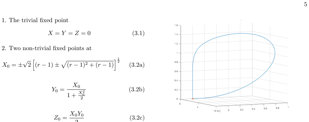
Two non-trivial fixed points at X0 =± √ 2 [ (r− 1)± √ (r− 1)2 + (r− 1) ] 1 2 (3.2a) Y0 = X0 1 + X 2 0 2 (3.2b) Z0 = X0Y0 2 (3.2c) The fixed point (3.1) corresponds to the state where there is no flow and a static concentration gradient exists be- tween the plates. Linearizing about this fixed point, we have the perturbations δX,δY,δZ follow the dynamics ˙δX =...
-
[5]
Fluid mechanics, Vol. 6 of A course of Theoretical Physics,
L. D. Landau and E. M. Lifshitz, “Fluid mechanics, Vol. 6 of A course of Theoretical Physics,” Pergamon Press, (1959)
work page 1959
-
[6]
D. Ruelle and F. Takens, “On the nature of turbulence,” Commun. Math. Phys. 20, 167 (1971) and 23, 343 (1971)
work page 1971
Show all 34 references
-
[7]
Occurrence of strange Axiom A attractors near quasi-periodic flows on Tm, m ≥ 3,
S. Newhouse, D. Rulle and F. Takens, “Occurrence of strange Axiom A attractors near quasi-periodic flows on Tm, m ≥ 3,” Commun. Math. Phys. 64, 35 (1978)
1978
-
[8]
Deterministic nonperiodic flow,
E. N. Lorenz, “Deterministic nonperiodic flow,” J. At- mos. Sc. 20, 130 (1963)
1963
-
[9]
Nonlinear dynamics and chaos,
See for e.g. S. H. Strogatz, “Nonlinear dynamics and chaos,” Westview Pres (2015)
2015
-
[10]
Quantitative universality for a class of nonlinear transformations,
M. J. Feigenbaum, “Quantitative universality for a class of nonlinear transformations,” J. Stat. Phys, 19, 25 (1978)
1978
-
[11]
Sensitive dependence to initial condi- tions for one-dimensional maps,
J. Guckenheimer, “Sensitive dependence to initial condi- tions for one-dimensional maps,” Comm. Math. Phys. 70 133 (1979)
1979
-
[12]
The onset spectrum of turbulence,
M. J. Feigenbaum, “The onset spectrum of turbulence,” Phys. Lett. A 74, 375 (1979)
1979
-
[13]
The behavior of nonlinear vibrating sys- tem,
W. S.-Stupica, “The behavior of nonlinear vibrating sys- tem,” Kluwer Academic, London (1990)
1990
-
[14]
Period dou- bling cascade in mercury, a quantitative measurement,
A. Libchaber, C. Laroche and S. Fauve, “Period dou- bling cascade in mercury, a quantitative measurement,” J. Physique Lett. 43, 211 (1982)
1982
-
[15]
The mechanics and statics of active matter,
S. Ramaswamy, “The mechanics and statics of active matter,” Ann. Rev. Condens. Matter Phys. 1, 323 (2010)
2010
-
[16]
Hydrodynamics of soft ac- tive matter,
M. C. Marchetti, J. F. Joanny, S. Ramaswamy, T. B.Liverpool, and J. Prost, “Hydrodynamics of soft ac- tive matter,” Rev. Mod. Phys. 85, 1143 (2013)
2013
-
[17]
Active suspensions and their nonlinear models,
D. Saintillan and M. Shelley, “Active suspensions and their nonlinear models,” Comptes Rendus Physique, 14, 497 (2013)
2013
-
[19]
Non- linear dynamics and rheology of active fluids: Simula- tions in two dimensions,
S. M. Fielding, D. Marenduzzo, and M. E. Cates, “Non- linear dynamics and rheology of active fluids: Simula- tions in two dimensions,” Phys. Rev. E 83, 041910 (2011)
2011
-
[21]
Instabilities, pattern for- mation, and mixing in active suspensions,
D. Saintillan and M. J. Shelley, “Instabilities, pattern for- mation, and mixing in active suspensions,” Phys. Fluids 20, 123304 (2008)
2008
-
[22]
Active model H: Scalar active matter in a momentum-conserving fluid,
A. Tiribocchi, R. Wittkowski, D.Marenduzzo, and M.Cates, “Active model H: Scalar active matter in a momentum-conserving fluid,” Phys. Rev. Lett. 115,8 188302 (2015)
2015
-
[23]
Theory of dynamic critical phenomena,
P. C. Hohenberg and B. I. Halperin, “Theory of dynamic critical phenomena,” Rev. Mod. Phys. 49, 435 (1977)
1977
-
[24]
Driven ac- tive matter: Fluctuations and a hydrodynamic instabil- ity,
T. R. Kirkpatrick and J. K. Bhattacherjee, “Driven ac- tive matter: Fluctuations and a hydrodynamic instabil- ity,” Phys. Rev. Fluids 4, 024306 (2019)
2019
-
[25]
Introduction to Nonlinear Mechanics,
N. M. Krylov and N. N. Bogolyubov, “Introduction to Nonlinear Mechanics,” Princeton University Press, Princeton (1947)
1947
-
[26]
Singular Perturbation Theory
D. Smith, “Singular Perturbation Theory”, Cambridge University Press, Cambridge (1985). 12
1985
-
[27]
The Lorenz equations: bifurcations, chaos, and strange attractors,
C. Sparrow, “The Lorenz equations: bifurcations, chaos, and strange attractors,” Springer-Verlag, New York (1982)
1982
-
[28]
Local and global behav- ior near homoclinic orbits,
P. Glendinning and C. Sparrow, “Local and global behav- ior near homoclinic orbits,” J. Stat. Phy. 35, 645 (1984)
1984
-
[29]
What can we learn from homoclinic orbits in chaotic dynamics?
P. Gaspard and G. Nicolis, “What can we learn from homoclinic orbits in chaotic dynamics?” J. Stat. Phy. 31, 499 (1984)
1984
-
[30]
Transition to turbu- lence in a statistically stressed fluid system,
J. B. McLaughlin and P. C. Martin, “Transition to turbu- lence in a statistically stressed fluid system,” Phys. Rev. A 12, 186-203 (1975)
1975
-
[31]
Super- critical and sub-critical Hopf bifurcations in two and three dimensions,
D. Das, D. Banerjee and J. K. Bhattacharjee, “Super- critical and sub-critical Hopf bifurcations in two and three dimensions,” Nonlinear Dynamics 77, 169-184 (2014)
2014
-
[32]
Fluid flocks with inertia,
R. Chatterjee, N. Rana, R. Aditi Simha, P. Perlekar and S. Ramaswamy, “Fluid flocks with inertia,” arXiv 1907.03492 (2019)
2019 arXiv
-
[33]
Hydrodynamically inter- rupted droplet growth in scalar active matter,
R. Singh and M. E. Cates, “Hydrodynamically inter- rupted droplet growth in scalar active matter,” arXiv 1907.04819 (2019)
2019 arXiv
-
[34]
Hydrodynamics of active defects: from order to chaos to defect ordering,
S. Shankar and M. Cristina Marchetti, “Hydrodynamics of active defects: from order to chaos to defect ordering,” arXiv 1907.02468 (2019)
2019 arXiv
Reviewed August 14, 2026 · model on record in the stance chip above.
Discussion (0). Continue with ORCID to comment.