REVIEW 3 major objections 5 minor 15 references
Bayesian posterior repartitioning for nested sampling
T0 review · 3 major / 5 minor · reviewed 2026-08-14 · deepseek-v4-flash
Pith's one-line read Treating the prior-repartitioning power β as a hyperparameter makes nested sampling self-adapting and correct even when the prior is unrepresentative.
desk verdict A conceptually simple and potentially useful extension of posterior repartitioning, but the paper's central factorization assumption is contradicted by its own asymmetric multimodal example, so treat the default-use claim with caution. read the letter →
The pith
A machine-rendered reading of the paper's core claim, the machinery that carries it, and where it could break.
The reading
What carries the argument
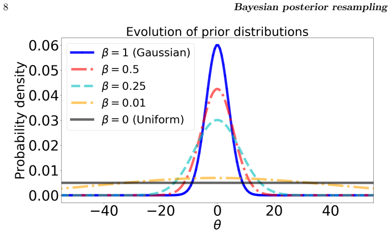
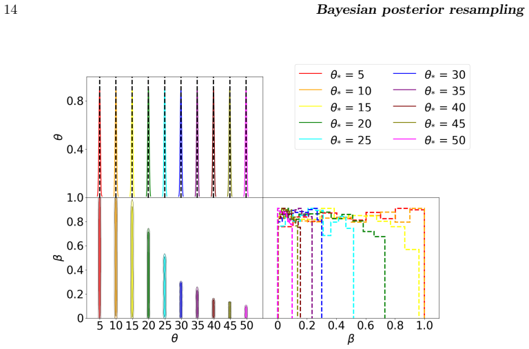
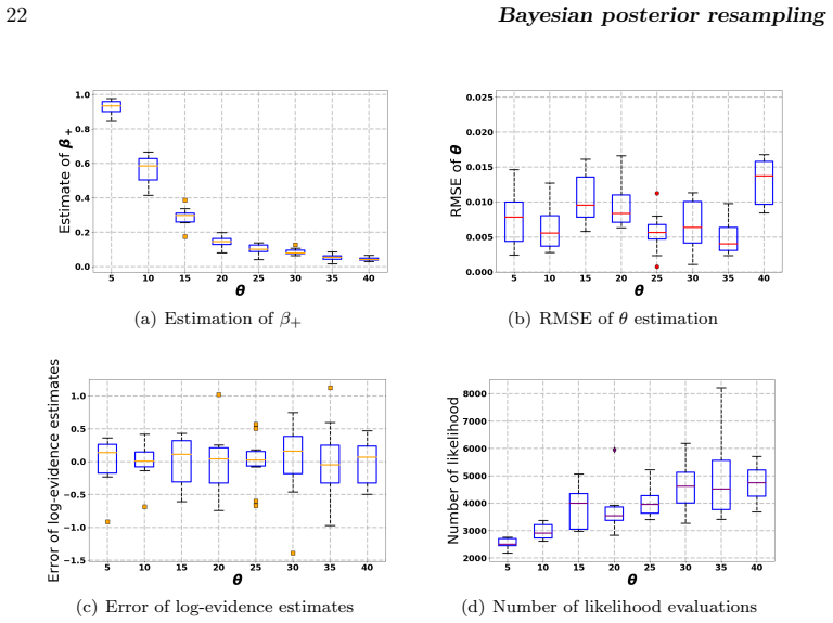
The load-bearing identity is the prior–likelihood repartitioning L(θ)π(θ) = L̃(θ,β)π̃(θ|β)π(β) with π̃(θ|β) ∝ π(θ)^β and β ∈ [0,1], which keeps the evidence fixed while broadening the effective prior. The method's second element is the effective posterior factorization: when the sampler fails for extreme β, the returned joint distribution is P(θ)P̃(β) rather than P(θ)π(β), and the marginal P̃(β) is a top-hat-like distribution over [β−,β+]. The third element is the histogram-scaling correction that converts the observed β marginal into an estimate of the missing mass, making the evidence estimate unbiased. Together these pieces let one extra hyperparameter absorb the failure mode of nested sampling with unrepresentative priors.
What would settle it
Run BPR on a constructed problem where the effective β marginal is not flat but strongly bimodal or concentrated near β+, and compare the histogram-corrected log-evidence with exact quadrature. If the correction uses only the largest bin, a visibly non-flat P̃(β) should produce a bias that grows with the departure from flatness; observing that bias would falsify the claim that the correction always recovers the evidence. Alternatively, a case where the sampler fails even at low β, so that no bin of P̃(β) reliably equals π(β), would violate the assumption.
Extended reading notes
Core claim
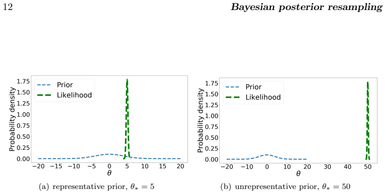
By construction, replacing the prior with π̃(θ|β) ∝ π(θ)^β and the likelihood with L̃(θ,β) = L(θ)π(θ)^(1−β)Z_π(β) keeps the product L(θ)π(θ) unchanged. Treating β as uniform on [0,1] and sampling the joint distribution therefore yields samples from P(θ)π(β); the marginal on θ is the original posterior exactly. In realistic finite-live-point runs with an unrepresentative prior, the sampler returns an effective posterior P(θ)P̃(β), where P̃(β) is nonzero only over [β−,β+]; marginalizing over θ still gives P(θ), so parameter inference is correct, and β+ diagnoses how far into the prior wings the likelihood lies. The paper's evidence correction scales the histogram of β samples so that its largest bin has the same integrated mass as the prior π(β) over that bin, then sums the bin volumes to estimate the missing-mass factor ∫P̃(β)dβ; this restores unbiased evidence estimates in all tested examples.
Load-bearing premise
The evidence correction assumes that, in the bin of the β histogram containing the most samples, the sampler is unbiased and the effective marginal P̃(β) equals the prior π(β), so scaling that bin to the prior's integrated mass correctly estimates the missing mass elsewhere; this is assumed rather than derived.
Editorial extensions
If this is right
- A single nested-sampling run with β added as a hyperparameter replaces the multiple runs and annealing schedule of the original PR method, cutting computational cost by orders of magnitude.
- Analyses on many datasets can use one standard prior without pre-screening: representative datasets pay negligible overhead, while unrepresentative ones are automatically handled and flagged.
- Multi-modal likelihoods whose modes lie at different distances from the prior centre can be sampled correctly in one run, because different β ranges are inferred for different regions.
- The upper edge β+ of the β marginal becomes a quantitative, self-calibrating measure of how unrepresentative a prior is for a given dataset.
- Evidence estimates remain accurate in the failure regime after the histogram correction, so model comparison is not corrupted by unrepresentative priors.
Reading between the lines
- β+ could be repurposed as a cheap outlier score in survey-scale pipelines: compute it per dataset and re-analyse only those with small values, rather than re-running every dataset.
- If β were given an informative prior instead of uniform, BPR could encode a preference for how aggressively to repartition, turning the method into a tunable shrinkage toward standard NS.
- The same joint-reparameterisation idea may transfer to any sampler that uses the prior and likelihood separately, not only to the specific nested-sampling implementation tested here.
- A natural further test is to verify that the histogram-scaling evidence correction remains unbiased when the effective β marginal has several modes, since the paper demonstrates multi-modal θ posteriors but only shows unimodal β marginals.
Signed reviews
Editorial analysis
A structured set of objections, weighed in public.
Referee Report
Summary. The paper proposes Bayesian posterior repartitioning (BPR), a method for making nested sampling (NS) more robust against unrepresentative priors. The key idea is to introduce an auxiliary hyperparameter β that controls a power transformation of the prior, and to treat β as an unknown to be sampled jointly with the original parameters θ in a single NS run. The authors show that, by construction, the joint posterior on (θ, β) is proportional to P(θ)π(β) (Eq. 10), so that marginalizing over β returns the original posterior P(θ) (Eq. 13) and the evidence is unchanged (Eq. 12). Recognizing that finite-Nlive NS may fail at extreme β values, they posit an 'effective posterior' factorized as P(θ)P~(β) (Eq. 15) and propose a histogram-based correction for the evidence (Eq. 16). Numerical experiments with MultiNest are presented for Gaussian, Laplace, and multimodal likelihoods from 1D to 10D, showing accurate parameter and evidence recovery relative to quadrature, and a negligible computational overhead for representative priors. The paper concludes that BPR should be used as the default in all NS analyses.
Significance. If the method holds up, BPR is a practically valuable contribution to the nested-sampling literature: it automates the choice of the power-prior exponent β, removes the annealing-schedule dependence of the earlier PR method, and offers a diagnostic (β+) for detecting unrepresentative priors. The exact construction in Eqs. (9)-(13) is correct and elegant, and the numerical validation is extensive for smooth unimodal targets. However, the central additional claims—that the effective posterior factorizes as in Eq. (15) and that the evidence correction in Eq. (16) is unbiased—are not established from first principles and are contradicted by the paper's own asymmetric multimodal example. The paper also overstates the robustness of BPR as a default method. Thus the contribution is promising but currently incomplete.
major comments (3)
- [Section 3, Eq. (15); Section 4.4, Fig. 13] The effective posterior factorization P~_eff(θ,β) ∝ P(θ)P~(β) in Eq. (15) implies that β and θ are independent under the sampling distribution. Yet Fig. 13(a)-(b) shows that, in the asymmetric 4-mode example, the mean log β differs strongly between modes 1/4 and modes 2/3 (by orders of magnitude in Fig. 13(b)). This is direct empirical evidence that the output of NS-BPR is not distributed as Eq. (15) in exactly the multi-modal, spatially asymmetric scenario advertised as a key advantage of BPR. Because the argument that marginalizing β over the effective posterior recovers P(θ) (the basis for the parameter-recovery claim) and the evidence correction in Eq. (16) both rely on Eq. (15), the paper's central practical claims are unsupported for this regime.
- [Section 3, Eq. (16) and surrounding discussion] The evidence correction in Eq. (16) is heuristic and is not derived from any stated principle. The procedure assumes that the histogram bin with the largest number of β samples corresponds to a region where the NS sampler is unbiased (P~(β)=π(β)), and then scales the histogram so that this bin has volume ∫β_l^β_u π(β)dβ. This is circular in the sense that the same samples used to construct the histogram are used to determine which bin is 'unbiased'. No convergence argument or error bound is given, and no test of the correction is presented for a case in which Eq. (15) is violated (e.g., the asymmetric multimodal example of Sec. 4.4). The evidence estimates in Tables 1, 3, and 4 are all consistent with quadrature, but those cases also exhibit the product form of Eq. (15); the correction's validity in the non-factorized regime is therefore untested.
- [Section 4.4, Fig. 13(c)-(f)] In the asymmetric arrangement, the default Nlive=100 yields large and volatile RMSE for modes 1 and 4 (Fig. 13(c)), and for the furthest mode centers the NS run produces no samples at all in those modes (Fig. 13(e)). The paper presents this as defining the limit of applicability, but it directly undermines the abstract's and Conclusion's claim that BPR 'allows' BPR to accommodate spatially asymmetric modes in a robust, hands-off manner. Since the negligible-overhead default-use claim is premised on Nlive=100, this is a load-bearing limitation rather than a minor caveat. The paper should either restrict the robustness claims to the symmetric case or provide a principled way to set Nlive for asymmetric problems.
minor comments (5)
- [Section 1, para. 2] Typo: 'settng β = 1' should read 'setting β = 1'.
- [Section 3, para. after Eq. (9)] Typo: 'movitation' should read 'motivation'.
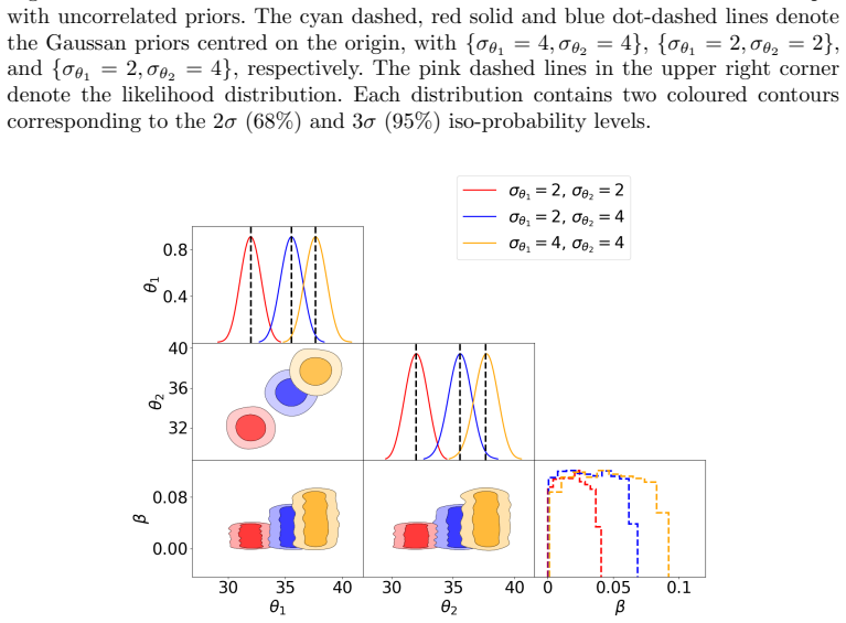
- [Figure 6 caption] The caption states the contours correspond to the '2σ (68%) and 3σ (95%)' iso-probability levels. For a Gaussian, 68% corresponds to 1σ and 95% to 2σ, so the percentages are misassigned.
- [Section 4.4, Figs. 12 and 13] The captions of Fig. 13 say 'As for Fig 12' while Fig. 12's caption says 'Performance of the BPR method applied to multimodal likelihoods...'; the wording should be made consistent and the differences (per-mode vs averaged quantities) clearly stated.
- [Section 3, Eq. (14)] The sentence 'one has neither gained nor lost anything by introducing the hyperparameter β' is true only if NS samples the exact joint posterior; this proviso should be restated directly before Eq. (14) to avoid confusion with the effective-posterior discussion that follows.
Circularity Check
BPR's posterior-recovery claim is true by construction, and its evidence correction self-normalizes to the prior; no load-bearing self-citation, and external benchmarks keep the circularity partial.
-
self definitional
[Section 3, Eqs. (9)-(13)]
"From the relations (6) and (2), one sees that (by construction) P~(θ,β) ∝ P(θ)π(β). ... Hence, ... by marginalising over β ... P~(θ)=∫P~(θ,β)dβ=∫P(θ)π(β)dβ=P(θ)."
The BPR joint posterior is introduced by defining the effective prior and likelihood so that their product equals L(θ)π(θ). Therefore Eq. (10) is an identity, not a sampler result: it says the joint posterior is proportional to the original posterior times the beta prior. Eq. (13) then merely integrates the beta prior to unity. The claim that marginalizing over beta recovers P(θ) is built into the construction, as the paper itself says 'by construction'. It is a restatement of the defining constraint used to build the joint distribution, not an independent prediction.
-
fitted input called prediction
[Section 3, Eq. (16) and following paragraph]
"this may be achieved by first scaling the distribution P~(β), represented as a histogram of equally-weighted posterior samples, such that the bin containing the largest number of samples has the volume ∫βu βl π(β)dβ ... The factor ∫P~(β)dβ may then be calculated by summing up the volumes of all the bins in the resulting scaled histogram."
The evidence-correction factor is not derived from NS dynamics; it is fitted by assuming that the effective beta-marginal equals the prior π(β) in the most populated bin. The corrected evidence is then normalized by that assumed equality: the factor ∫P~(β)dβ is the prior mass in that bin divided by the sample fraction in that bin. Thus the correction is a self-calibration of the very samples it corrects, and the recovered evidence is forced, by construction, to be consistent with the prior mass in that bin. The agreement with quadrature is an external check, not an internal derivation.
full rationale
The derivation chain contains two genuinely definitional/fitted steps. First, the BPR joint posterior is assembled by choosing effective prior and likelihood whose product is L(θ)π(θ); Eqs. (10)-(13) then immediately give the original posterior after marginalizing β, and the paper even says 'by construction', so this is not an independent result. Second, the finite-N evidence correction in Section 3 sets the normalization of the empirical β-histogram by requiring its largest bin to have the prior volume over that bin; the correction factor is then read off from that same scaled histogram, so the corrected evidence is calibrated to the assumption that the sampler is unbiased in the most populated bin. These two steps justify the partial circularity score. The paper's numerical comparisons with quadrature evidence and known Gaussian posteriors are external, reproducible checks, so the circularity is not total. Self-citations to Chen et al. (2018) and Feroz et al. (2009) are not load-bearing here: they support the original PR method and the NS implementation, not the BPR identity. I also note that the paper's Section 4.4 asymmetric multimodal example reports mode-dependent β values, which appears inconsistent with the factorization in Eq. (15); that is a correctness risk rather than a circularity, so it does not raise the circularity score further. The paper itself concedes 'there is a paucity of further theoretical arguments from which to predict the form of P~(β)', confirming that the histogram scaling is an assumption rather than a derived result.
Assumptions & free parameters
assumptions (5)
- standard math Bayes' theorem and the nested sampling algorithm (Skilling 2006) provide unbiased estimates in the large-Nlive limit.
- domain assumption The normalization constant Zpi(beta)=integral pi(theta)^beta dtheta is known or computable for the priors used.
- domain assumption The prior on beta is uniform on [0,1].
- ad hoc to paper For finite Nlive, the actual sampling distribution factorizes as P_eff_tilde(theta,beta) proportional to P(theta) P_tilde(beta), with P_tilde(beta) non-zero only over [beta-, beta+].
- ad hoc to paper The histogram bin with the largest number of beta samples corresponds to unbiased sampling where P_tilde(beta)=pi(beta).
invented entities (2)
-
Effective posterior P_eff_tilde(theta,beta)
-
Effective evidence Z_eff_tilde
Cite this review
Pith. "Pith review of Bayesian posterior repartitioning for nested sampling." pith.science (2026). https://pith.science/paper/I4HFXJZP
@misc{pith2026190804655,
  author       = {Pith},
  title        = {Pith review of: Bayesian posterior repartitioning for nested sampling},
  year         = {2026},
  howpublished = {\url{https://pith.science/paper/I4HFXJZP}},
  note         = {Machine review of arXiv:1908.04655}
}
read the original abstract
Priors in Bayesian analyses often encode informative domain knowledge that can be useful in making the inference process more efficient. Occasionally, however, priors may be unrepresentative of the parameter values for a given dataset, which can result in inefficient parameter space exploration, or even incorrect inferences, particularly for nested sampling (NS) algorithms. Simply broadening the prior in such cases may be inappropriate or impossible in some applications. Hence our previous solution to this problem, known as posterior repartitioning (PR), redefines the prior and likelihood while keeping their product fixed, so that the posterior inferences and evidence estimates remain unchanged, but the efficiency of the NS process is significantly increased. In its most practical form, PR raises the prior to some power beta, which is introduced as an auxiliary variable that must be determined on a case-by-case basis, usually by lowering beta from unity according to some pre-defined `annealing schedule' until the resulting inferences converge to a consistent solution. Here we present a very simple yet powerful alternative Bayesian approach, in which beta is instead treated as a hyperparameter that is inferred from the data alongside the original parameters of the problem, and then marginalised over to obtain the final inference. We show through numerical examples that this Bayesian PR (BPR) method provides a very robust, self-adapting and computationally efficient `hands-off' solution to the problem of unrepresentative priors in Bayesian inference using NS. Moreover, unlike the original PR method, we show that even for representative priors BPR has a negligible computational overhead relative to standard nesting sampling, which suggests that it should be used as the default in all NS analyses.
Figures

Figures from the paper (12 more)






Reference graph
Works this paper leans on
-
[1]
Statistics and Computing pp 1--16
Chen X, Hobson M, Das S, Gelderblom P (2018) Improving the efficiency and robustness of nested sampling using posterior repartitioning. Statistics and Computing pp 1--16
work page 2018
-
[2]
Monthly Notices of the Royal Astronomical Society 384(2):449--463
Feroz F, Hobson M (2008) Multimodal nested sampling: an efficient and robust alternative to Markov Chain Monte Carlo methods for astronomical data analyses . Monthly Notices of the Royal Astronomical Society 384(2):449--463
work page 2008
-
[3]
Monthly Notices of the Royal Astronomical Society 398(4):1601--1614
Feroz F, Hobson M, Bridges M (2009) MultiNest: an efficient and robust Bayesian inference tool for cosmology and particle physics . Monthly Notices of the Royal Astronomical Society 398(4):1601--1614
work page 2009
-
[4]
Feroz F, Hobson M, Cameron E, Pettitt A (2013) Importance nested sampling and the MultiNest algorithm . arXiv preprint arXiv:13062144
work page 2013
-
[5]
Handley W (2019) anesthetic: nested sampling visualisation. The Journal of Open Source Software 4(37), doi:10.21105/joss.01414, ://dx.doi.org/10.21105/joss.01414
-
[6]
Monthly Notices of the Royal Astronomical Society 453(4):4384--4398
Handley W, Hobson M, Lasenby A (2015) POLYCHORD: next-generation nested sampling . Monthly Notices of the Royal Astronomical Society 453(4):4384--4398
work page 2015
-
[7]
Statistics and Computing doi:10.1007/s11222-018-9844-0, ://doi.org/10.1007/s11222-018-9844-0
Higson E, Handley W, Hobson M, Lasenby A (2018) Dynamic nested sampling: an improved algorithm for parameter estimation and evidence calculation. Statistics and Computing doi:10.1007/s11222-018-9844-0, ://doi.org/10.1007/s11222-018-9844-0
-
[8]
MacKay D (2003) Information theory, inference and learning algorithms. Cambridge university press
work page 2003
Show all 15 references
-
[9]
Bayesian Analysis 1(4):833--860
Skilling J (2006) Nested Sampling for General Bayesian Computation . Bayesian Analysis 1(4):833--860
2006
-
[10]
, " * write output.state after.block = add.period write newline
ENTRY address archive author booktitle chapter doi edition editor eid eprint howpublished institution journal key month note number organization pages publisher school series title type url volume year label extra.label sort.label short.list INTEGERS output.state before.all mi...
-
[11]
write newline
" write newline "" before.all 'output.state := FUNCTION add.period duplicate empty 'skip "." * add.blank if FUNCTION if.digit duplicate "0" = swap duplicate "1" = swap duplicate "2" = swap duplicate "3" = swap duplicate "4" = swap duplicate "5" = swap duplicate "6" = swap dupl...
-
[12]
, " * write output.state after.block = add.period write newline
ENTRY address author booktitle chapter doi edition editor eid howpublished institution journal key month note number organization pages publisher school series title type url volume year label INTEGERS output.state before.all mid.sentence after.sentence after.block FUNCTION in...
-
[13]
write newline
" write newline "" before.all 'output.state := FUNCTION if.digit duplicate "0" = swap duplicate "1" = swap duplicate "2" = swap duplicate "3" = swap duplicate "4" = swap duplicate "5" = swap duplicate "6" = swap duplicate "7" = swap duplicate "8" = swap "9" = or or or or or or...
-
[14]
, " * write output.state after.block = add.period write newline
ENTRY address author booktitle chapter doi edition editor eid howpublished institution journal key month note number organization pages publisher school series title type url volume year label INTEGERS output.state before.all mid.sentence after.sentence after.block FUNCTION in...
-
[15]
write newline
" write newline "" before.all 'output.state := FUNCTION if.digit duplicate "0" = swap duplicate "1" = swap duplicate "2" = swap duplicate "3" = swap duplicate "4" = swap duplicate "5" = swap duplicate "6" = swap duplicate "7" = swap duplicate "8" = swap "9" = or or or or or or...
Reviewed August 14, 2026 · model on record in the stance chip above.
Discussion (0). Continue with ORCID to comment.