REVIEW 2 major objections 5 minor 23 references
A computational approach for the study of electromagnetic interactions in reacting flows
T0 review · 2 major / 5 minor · reviewed 2026-08-15 · deepseek-v4-flash
Pith's one-line read EMI-SENGA solves Maxwell's equations with compressible reacting flows, so Lorentz, polarization, and magnetization forces alter momentum, species diffusion, and energy while the medium's properties reshape the fields in return.
desk verdict Novel FDTD–DNS coupling with solid partial validations, but the §2.1.2 charge-conservation argument fails and the coupled EM results are not yet trustworthy. read the letter →
The pith
A machine-rendered reading of the paper's core claim, the machinery that carries it, and where it could break.
The reading
What carries the argument
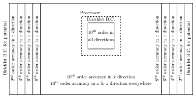
The framework rests on three coupled pieces of machinery. The first is a Gauss-law potential solver for electrostatic and magnetostatic fields, which keeps the susceptibility-gradient terms in the potential equations that earlier formulations typically dropped. The second is an FDTD wave solver on a staggered Yee cell that advances Ampere's and Faraday's laws at its own much smaller timestep, surrounded by CPML absorbing layers and fed by a soft Hertzian-dipole source. The third is the force feedback loop: the Lorentz, polarization, and magnetization forces (the last in Gilbert's separated-charge form) are inserted as volume forces and drift velocities into the momentum, species, and energy equations, and the resulting conductivity and charge distribution feed the next field update. The identity that keeps the two sides consistent is charge conservation, which guarantees that once the initial electric field is set from Gauss's law, the FDTD update preserves $\nabla\cdot\mathbf{E} = \rho_q/\epsilon_0$ throughout the simulation.
What would settle it
Probe the electric-field profile and ion current in a burner-stabilized methane-air flame under a known DC potential: the FDTD mode of EMI-SENGA predicts the field inside the reaction zone is measurably reduced within about 10 ns when the electron mobility is near $0.2\ \mathrm{m^2/(V\,s)}$, whereas the electrostatic mode predicts no such change, so a measurement combined with an independently determined electron mobility settles whether the induced-current feedback is real.
Extended reading notes
Core claim
On the authors' own terms, the central claim is that electromagnetic interactions in reacting flows can be represented faithfully in one DNS framework by solving Maxwell's equations and the flow conservation equations as a single coupled system, rather than imposing static fields as prior studies did. The Lorentz force on ions and electrons, the polarization force on polar and polarizable neutrals, and the magnetization force on species with net spin all enter the momentum, species-diffusion, and energy equations as volume forces and drift terms, while the species in turn determine the medium's permittivity (through the Clausius-Mossotti relation), conductivity (through mobility-weighted charge densities), and permeability (through Curie-law and Stoner susceptibilities), feeding back into the fields. In the cases computed — external potentials up to 900 V, magnetostatic potentials up to 20 kA, and a 100 GHz sinusoidal source — the framework reproduces ion accumulation and oxygen-anion generation near the inlet, shows that uniform magnetic fields barely disturb the flame while field gradients bend it (2–26 K of temperature variation), and shows that at electron mobilities near $0.2\ \mathrm{m^2/(V\,s)}$ the currents induced by moving charges alter the electric field in a way the electrostatic approximation misses entirely.
Load-bearing premise
The load-bearing premise is that the reacting medium is linear, isotropic, and nondispersive, so electrical permittivity and magnetic permeability are scalar fields independent of field strength, direction, and frequency; the authors state this can fail for high-strength waves, specific wavelengths, or particulate-laden reacting flows, and in those regimes both the wave propagation and the force predictions would require a more general constitutive model.
Editorial extensions
If this is right
- In ionized flames with high mobility, the electrostatic approximation fails: the paper's FDTD runs show induced currents modify the electric field even without an external source, so quasi-static codes miss part of the electrodynamics.
- The magnetic-susceptibility-gradient contribution to the magnetization force is comparable to the field-gradient contribution for weak fields, so dropping it, as earlier magnetostatic studies did, is not safe.
- Inhomogeneous magnetostatic boundary conditions deform the flame front, with 2–26 K of temperature variation across the flame in the tested 2D cases, so accurate magnetic boundary conditions matter for predicting field effects.
- High-frequency wave sources make the forces on electrons oscillatory and spatially patterned — above $10^{10}$ N/kg away from the source — so electron dynamics in such fields cannot be assumed to follow static-field logic.
- Because polarization and susceptibility terms are retained throughout, the framework extends unchanged to flows seeded with strongly polarizable or magnetizable particles, such as nanomaterials.
Reading between the lines
- These are my inferences, not the paper's claims: the same two-way coupling could replace the quasi-static electron treatment in plasma-assisted combustion and microwave-ignition models, where conductivity and electron-mobility feedback are suspected to control where energy is deposited.
- The appendix shows Gilbert's and Ampere's magnetization force models differ by a factor of two in the magnetostatic limit with small susceptibilities; a deflection measurement of a paramagnetic oxygen jet in a known field gradient would discriminate the two models.
- The paper's sensitivity runs show that the predicted field modification depends strongly on the assumed electron mobility (0.2 vs 0.01 m²/(V·s) changes the conductivity qualitatively), so the framework's predictive power at flame conditions hangs on pinning down this open transport input.
- The validation shows noticeable sensitivity of absorption quality to the CPML parameters, suggesting that reacting-flow FDTD applications will need case-specific absorbing-layer tuning.
Signed reviews
Editorial analysis
A structured set of objections, weighed in public.
Referee Report
Summary. The manuscript presents EMI-SENGA, an extension of the SENGA DNS code for simulating electromagnetic interactions in compressible reacting flows. Static electric and magnetic fields are obtained by solving Gauss's laws in potential form, while time-dependent electromagnetic waves are propagated with an explicit FDTD method. The Maxwell equations are coupled to the Navier-Stokes equations through Lorentz, polarization, and magnetization forces, with species transport augmented by field-dependent diffusion velocities. The solver is validated against Cantera for ionic species in a one-dimensional methane-air flame, against the analytical Hertzian-dipole solution of Ziolkowski et al. for FDTD wave propagation, and against gprMax for CPML absorbing boundary behavior. The capabilities are demonstrated for laminar flames under electrostatic, magnetostatic, and 100 GHz wave sources.
Significance. If the proposed formulation were fully consistent, EMI-SENGA would be a valuable, open-ended platform for studying electric- and magnetic-field control of combustion, including ionic wind, flame deformation by field gradients, and wave-flame interactions. The paper's strengths include a self-contained derivation of the force and drift-velocity models, a careful validation chain against independent codes (Cantera, gprMax) and an analytical solution, and an explicit sensitivity study of the electron-mobility parameter. The central weakness identified in this review is the claimed charge conservation of the FDTD coupling in reacting flows; until that point is resolved, the time-dependent results in Sections 3.6 and 3.7 should be interpreted with caution.
major comments (2)
- [2.1.2, Eq. (15)] The argument that Gauss's law remains satisfied is not valid. The FDTD update uses J = σ_e E (Eq. (7)), which omits the convective current ρ_q u and the diffusive current Σ_s q_s ρ Y_s V_s. The continuity equation imposed in the DNS is total-mass continuity; summing the species equations yields ∂ρ_q/∂t + ∇·(ρ_q u + Σ_s q_s ρ Y_s V_s) = 0, which is not equivalent to Eq. (15) with J = σ_e E. Consequently, there is no reason for ∇·D = ρ_q to hold after the E-field update, and the references [34,35] on rigorous charge conservation do not apply because the current is not derived from the charge motion. This affects the coupled FDTD results, especially Section 3.6 where the σ=0 test shows E unchanged despite evolving ρ_q; this is a symptom of the missing charge-flux coupling rather than evidence that currents are solely responsible. Please either include the full current in Ampere's law, or add a charge-conservation correction or error control, or otherwise demonstrate that the missing terms are negligible for the reported cases.
- [2.2, Eqs. (19)-(21) and Appendix A] As printed, the polarization and magnetization force expressions appear dimensionally inconsistent. For example, Eq. (19) gives f_P^s = ε0 ρ Y_s χ_e (E·∇)E, which has units of N·kg/m^6 rather than N/kg. The derivation in Appendix A (from Eq. (A.4) to Eq. (A.5)) indicates that the density ρ Y_s should divide, not multiply, the susceptibility term. If the typesetting is wrong, please correct it; if the solver implements the printed forms, the reported force magnitudes and the conclusions about the relative importance of polarization and magnetization forces (e.g., Section 3.2) need to be re-evaluated.
minor comments (5)
- [3.5, Fig. 14] The statement that the numerical and analytical solutions "perfectly overlap" should be quantified with an error norm (e.g., L2 relative error over the simulated time) to support the validation claim.
- [2.1.2] The FDTD update equations are not given in the paper but are referenced to Ref. [33], the first author's thesis; including the update stencils in an appendix or citing a public textbook page would improve accessibility.
- [3.6, Fig. 17] The units of the electric field in Fig. 17 are given as "V/Å", which appears to be a typo; likely the intended units are V/m or kV/m.
- [2.5] The boundary-condition bullets contain a typo: "if V_s^drift,i < 0 and |V_s^drift,i > u_i + V_s^Fick,i|" is missing a closing absolute-value bar, and the second bullet should state the Neumann condition more explicitly as ∂Y_s/∂x_i = 0.
- [B] In the derivation of Eq. (B.5), the neglect of the gradient of the average molecular weight is not stated until after Eq. (B.2); this assumption should be listed explicitly among the assumptions to avoid confusion.
Circularity Check
No significant circularity: the electromagnetic–reacting-flow solver is built from standard Maxwell and conservation equations, externally validated against analytical and independent numerical benchmarks; only a minor, non-load-bearing self-citation appears.
full rationale
The central derivation is self-contained. The electrostatic and magnetostatic solvers solve Eqs. (11)-(14), obtained by substituting the constitutive relations into Gauss's laws, and the FDTD wave solver is the standard Yee discretization of Ampere's and Faraday's laws, validated in Section 3.5 against the analytical Hertzian-dipole solution of Ref. [60] and against gprMax [61]. The reacting-flow coupling uses written-out conservation equations (Section 2.3) and derived force expressions (Appendices A-B); all material parameters (mobility, polarizabilities, susceptibilities, chemical mechanism) are independent literature inputs, not fitted to the outputs. The only self-citation is Ref. [33], the first author's PhD thesis, used for the EMI-FDTD update equations and CPML details, but these are standard FDTD formulae and the solver is externally benchmarked, so the citation is not load-bearing and no predicted quantity reduces to an input by construction. One non-circular caveat: the Section 2.1.2 assertion that Eq. (15) holds because 'the continuity equation is imposed in the DNS code and the chemical mechanism used in this study conserves the charges in the reactions' conflates total-mass continuity with the charge conservation needed for an FDTD update using J = sigma_e E; this is a physical consistency concern, not a circularity of the derivation chain.
Assumptions & free parameters
free parameters (1)
- Electron mobility mu_e- =
0.2 m^2/(V s), with an alternative 1 cm^2/(V s) from Belhi et al. tested in Section 3.6
assumptions (5)
- domain assumption The reacting medium is linear, isotropic, and nondispersive, so permittivity and permeability are scalar fields independent of field strength, direction, and frequency.
- domain assumption Charge conservation holds throughout the DNS via the continuity equation and a chemical mechanism that conserves charge.
- domain assumption Magnetostatic simulations may use the scalar magnetic potential H = -grad(Psi), which requires negligible electric current density.
- domain assumption Paramagnetic susceptibilities follow Curie's law with spin-only angular momentum (J approximately S), and diamagnetic susceptibilities are fixed literature values.
- domain assumption The free-electron magnetic susceptibility is described by the Stoner formula in the high-temperature limit epsilon_F/(k_B T) << 1.
Cite this review
Pith. "Pith review of A computational approach for the study of electromagnetic interactions in reacting flows." pith.science (2026). https://pith.science/paper/I4RKALET
@misc{pith2026250506433,
  author       = {Pith},
  title        = {Pith review of: A computational approach for the study of electromagnetic interactions in reacting flows},
  year         = {2026},
  howpublished = {\url{https://pith.science/paper/I4RKALET}},
  note         = {Machine review of arXiv:2505.06433}
}
read the original abstract
A computational fluid dynamics methodology for the simulation of electromagnetic interactions in compressible reacting flows has been formulated. The developed code, named EMI, is based on the SENGA Direct Numerical Simulation (DNS) software. Static electric and magnetic fields are solved using Gauss's laws of Maxwell's equations. Electromagnetic wave propagation is solved by discretizing Ampere's and Faraday's equations using the explicit Finite-Difference Time-Domain (FDTD) method. The equations for the electromagnetic fields are fully coupled with the Navier-Stokes equations, such that interactions between the electromagnetic fields and the fluid are included in the formulation. The interaction terms include the Lorentz, polarization, and magnetization forces. These forces determine volume forces that affect the transport of momentum, the diffusion velocity, and the energy conservation equations. In addition, the medium's properties affect the propagation of the electromagnetic fields via electrical permittivity and conductivity, charge density, and magnetic permeability. The solution of electromagnetic fields is validated against analytical and numerical solutions. The implementation of the coupling between electromagnetic fields and conservation equations for species, energy, and momentum is validated with laminar reacting flow numerical solutions from the literature. The capabilities of the formulation are investigated for a range of laminar methane-air computations under electrostatic, magnetostatic, and high-frequency electromagnetic waves. The validity of the electrostatic formulation in the presence of currents related to the movement of charged species is also assessed. Results demonstrate that EMI-SENGA can capture the fundamental effects of electromagnetic fields on reacting flows and the dynamics of charged species and their effect on flame shape and reactivity.
Figures


Figures from the paper (18 more)


Reference graph
Works this paper leans on
-
[1]
K. W. Jenkins, R. S. Cant, Direct numerical simulation of tu rbulent flame kernels, in: Recent Advances in DNS and LES: Proceedings of the Second AFOSR Conference held at Rutgers—The State University of New Jer sey, New Brunswick, USA, June 7–9, 1999, Springer, 1999, pp. 191–202
work page 1999
-
[2]
S. Cant, Direct numerical simulation of premixed turbul ent flames, Philo- sophical Transactions of the Royal Society of London. Serie s A: Mathe- matical, Physical and Engineering Sciences 357 (1764) (199 9) 3583–3604
-
[3]
E. Anderson, Z. Bai, C. Bischof, S. Blackford, J. Demmel, J. D ongarra, J. Du Croz, A. Greenbaum, S. Hammarling, A. McKenney, D. Sorensen, LAPACK Users’ Guide, 3rd Edition, Society for Industrial and Ap plied Mathematics, Philadelphia, PA, 1999
work page 1999
-
[4]
E. M. Kritikos, Electromagnetic fields and nanoenergeti c particles in re- acting flows, Ph.D. thesis, Imperial College London (2023)
work page 2023
- [5]
- [6]
-
[7]
A. Z. Elsherbeni, V. Demir, The Finite-Difference Time-Domai n: Method for Electromagnetics with MATLAB Simulations, 2nd Edition, ACES Se- ries on Computaional Electromagnetics and Engineering, Sc iTech Pub- lishing, an imprint of the IET, Edison, NJ, 2016
work page 2016
-
[8]
T. N. Olney, N. M. Cann, G. Cooper, C. E. Brion, Absolute scale de- termination for photoabsorption spectra and the calculati on of molecular properties using dipole sum-rules, Chemical Physics 223 (1 ) (1997) 59–98. doi:10.1016/S0301-0104(97)00145-6
Show all 23 references
-
[9]
T. M. Miller, B. Bederson, Atomic and Molecular Polariza bilities-A Re- view of Recent Advances, in: D. R. Bates, B. Bederson (Eds.), Ad vances in Atomic and Molecular Physics, Vol. 13, Academic Press, 197 8, pp. 1–55. doi:10.1016/S0065-2199(08)60054-8
-
[10]
B. I. Loukhovitski, A. S. Sharipov, A. M. Starik, Influence of vibrations and rotations of diatomic molecules on their physical prope rties: I. Dipole moment and static dipole polarizability, Journal of Physics B: Atomic, Molecular and Optical Physics 49 (12) (2016) 125102. doi...
2016
-
[11]
P. A. Gigu` ere, Molecular association and structure of h ydrogen peroxide, Journal of Chemical Education 60 (5) (1983) 399. doi:10.1021 /ed060p399
1983
-
[12]
D. Hait, M. Head-Gordon, How accurate are static polarizab ility predic- tions from density functional theory? An assessment over 132 species at equilibrium geometry, Physical Chemistry Chemical Phys ics 20 (30) (2018) 19800–19810. doi:10.1039/C8CP03569E
2018 doi
-
[13]
Gussoni, M
M. Gussoni, M. Rui, G. Zerbi, Electronic and relaxation contribu- tion to linear molecular polarizability. An analysis of the e xperimen- tal values, Journal of Molecular Structure 447 (3) (1998) 163 –215. doi:10.1016/S0022-2860(97)00292-5
1998 doi
-
[14]
W. M. Haynes, D. R. Lide, T. J. Bruno, CRC Handbook of Chemistr y and Physics, CRC press, 2016
2016
-
[15]
R. J. Kee, F. M. Rupley, E. Meeks, J. A. Miller, Chemkin-iii: A for- tran chemical kinetics package for the analysis of gas-phas e chemical and plasma kinetics, Tech. rep., Sandia National Lab.(SNL-CA), Li vermore, CA (United States) (1996). 21
1996
-
[16]
R. J. Kee, G. Dixon-Lewis, J. Warnatz, M. E. Coltrin, J. A. Mil ler, A fortran computer code package for the evaluation of gas-ph ase mul- ticomponent transport properties, Sandia National Laborat ories Report SAND86-8246 13 (1986) 80401–1887
1986
-
[17]
D. G. Goodwin, R. L. Speth, H. K. Moffat, B. W. Weber, Cantera : An Object-oriented Software Toolkit for Chemical Kinetics, T hermodynam- ics, and Transport Processes (2018). URL https://www.cantera.org
2018
-
[18]
Selle, U
S. Selle, U. Riedel, Transport Properties of Ionized Spe cies, Annals of the New York Academy of Sciences 891 (1) (1999) 72–80. doi:10.1111 /j.1749- 6632.1999.tb08754.x
1999
-
[19]
Selle, U
S. Selle, U. Riedel, S. Selle, U. Riedel, T. T. K, Transport Coefficients of Reacting Air at High Temperatures (2000)
2000
-
[20]
R. V. Chiflikian, The analog of Blanc’s law for drift veloc ities of electrons in gas mixtures in weakly ionized plasma, Physics of Plasmas 2 (10) (1995) 3902–3909. doi:10.1063/1.871019
1995 doi
-
[21]
L. A. Viehland, E. A. Mason, W. F. Morrison, M. R. Flannery, Table s of transport collision integrals for (n, 6, 4) ion-neutral p otentials, Atomic Data and Nuclear Data Tables 16 (6) (1975) 495–514. doi:10.10 16/0092- 640X(75)90022-4
1975
-
[22]
Prager, Modeling and Simulation of Charged Species in Lean Methane-Oxygen Flames, https://archiv.ub.uni-heidelberg.de/volltextserver/5889/ (2005)
J. Prager, Modeling and Simulation of Charged Species in Lean Methane-Oxygen Flames, https://archiv.ub.uni-heidelberg.de/volltextserver/5889/ (2005). doi:10.11588/heidok.00005889
2005 doi
-
[23]
R. W. Ziolkowski, N. K. Madsen, R. C. Carpenter, Three-dim ensional computer modeling of electromagnetic fields: A global lookb ack lattice truncation scheme, Journal of Computational Physics 50 (3) ( 1983) 360– 408. 22
1983
Reviewed August 15, 2026 · model on record in the stance chip above.
Discussion (0). Continue with ORCID to comment.