REVIEW 3 major objections 5 minor 15 references
Estimation methods of Matrix-valued AR model
T0 review · 3 major / 5 minor · reviewed 2026-08-07 · deepseek-v4-flash
Pith's one-line read Adapted Yule-Walker and Burg estimators give matrix-valued autoregressive models predictive accuracy comparable to VAR at a fraction of the parameters.
desk verdict The Burg estimator has a false convexity proof and the simulations only test B=I, but the YW half is sound and the topic is worth refereeing. read the letter →
The pith
A machine-rendered reading of the paper's core claim, the machinery that carries it, and where it could break.
The reading
What carries the argument
The load-bearing object is the Burg prediction-error objective, $E_k(A,B)=\sum_{t=k+1}^N\left(\|f_t^{(k-1)}-A b_{t-1}^{(k-1)}B^T\|_F^2 + \|b_{t-1}^{(k-1)}-A f_t^{(k-1)}B^T\|_F^2\right)$, together with the Kronecker identity $\mathrm{vec}(AXB^T)=(B\otimes A)\mathrm{vec}(X)$ that turns matrix operations into standard linear algebra. The Yule-Walker side uses Kronecker-structured autocovariance matrices $\Gamma_i^\otimes=E[X_t\otimes X_{t-i}^T]$, whose entries are permutations of the usual vector autocovariances; the estimator minimizes the Frobenius residual of $\Gamma_1^\otimes = (A\otimes I_n)\Gamma_0^\otimes(B^T\otimes I_m)$ under $\|A\|_F=1$. These objects carry the argument by converting a bilinear estimation problem into a sequence of least-squares steps that can be solved alternately for one coefficient matrix while the other is fixed.
What would settle it
Take the scalar case $f_t=1$, $b_t=2$: the Burg objective reduces to $E(A,B)=(1-2AB)^2+(2-AB)^2$. At $A=B=1$ the Hessian has determinant $-44$, so the objective is not jointly convex; running the alternating updates from many random starts on a small simulated series and comparing the resulting objective values would show whether the method misses lower-error solutions.
Extended reading notes
Core claim
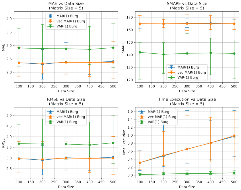
At the mathematical core, the paper argues that the Kronecker product lets classical autocovariance-based estimators carry over to matrix-valued series. For the MAR(1) model $X_t = A X_{t-1}B^T + Z_t$ with $\|A\|_F=1$, the Yule-Walker equations take the Kronecker form $\Gamma_1^\otimes = (A\otimes I_n)\Gamma_0^\otimes(B^T\otimes I_m)$, and the paper estimates $A,B$ by minimizing the Frobenius distance of this equation, a nearest-Kronecker-product problem. For Burg's method, the paper defines forward residuals $f_t^{(k)}$ and backward residuals $b_t^{(k)}$, derives the recursions $f_t^{(k)} = f_t^{(k-1)} - A_k(k)b_{t-1}^{(k-1)}B_k(k)^T$ and $b_t^{(k)} = b_{t-1}^{(k-1)} - A_k(k)f_t^{(k-1)}B_k(k)^T$, and minimizes the summed squared norms by alternating closed-form updates in $A$ and $B$, with higher-order lags handled by a Levinson-type recursion and a nearest-Kronecker step. The paper claims (Theorem B2) that this alternating solution is a global minimum because the objective is jointly convex. Empirically, the paper reports that MAR models estimated this way match VAR on MAE and RMSE in the simulated experiments while using many fewer parameters.
Load-bearing premise
The proof that the Burg estimator reaches the globally best coefficients assumes the error surface has a single bowl shape in both coefficient matrices at once; if the surface instead has several dips, the alternating updates can settle in a dip that is not the deepest.
Editorial extensions
If this is right
- Practitioners can fit MAR(1) models to large matrix time series and obtain MAE and RMSE on par with VAR(1) while estimating $m^2+n^2$ coefficients instead of $m^2n^2$.
- Because Yule-Walker and Burg estimators are built from autocovariances, fitted MAR models preserve the autocorrelation structure and, under $\rho(A)\rho(B)<1$, are causal, avoiding a known failure mode of LSE and MLE fits.
- The Levinson-type recursion extends the Burg estimator beyond first order, so the method supplies MAR($p$) estimates rather than only MAR(1).
- Mardia's test results reported in the paper indicate approximately multivariate normal residuals for most simulated fits, supporting the white-noise assumptions used to derive the estimators.
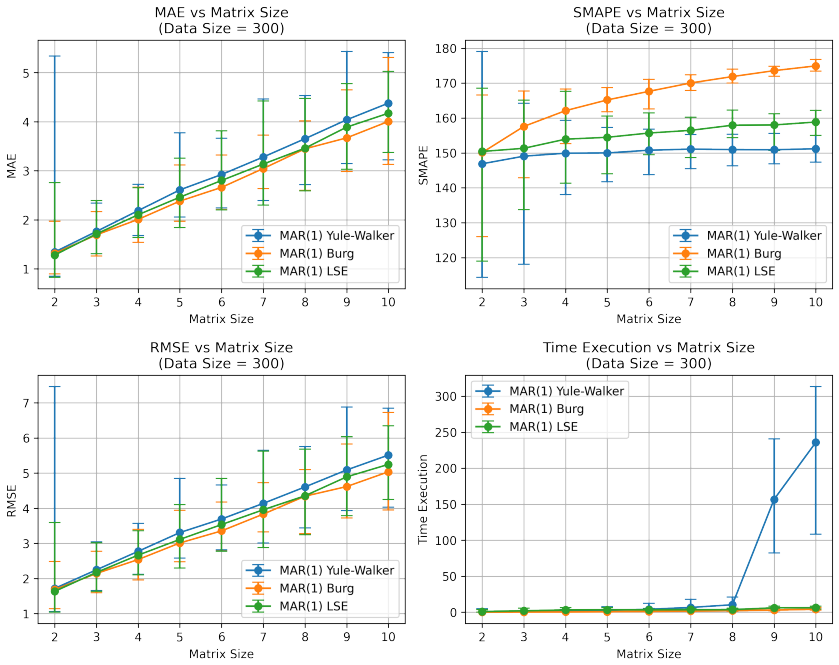
- Burg's method is reported to be consistently fast across the simulated settings, whereas the Yule-Walker approach slows sharply as matrix dimension grows.
Reading between the lines
- The global-minimum claim in Theorem B2 rests on joint convexity of the Burg objective, but a squared Frobenius norm of a bilinear expression is not jointly convex in general; consequently a convergence or multi-start analysis, which the paper does not report, is needed to know whether the alternating updates find the best coefficients.
- The nearest-Kronecker-product subproblems in both estimators could be solved by alternating least squares with closed-form updates, potentially making the Yule-Walker method much faster than the L-BFGS-B optimization used in the paper.
- The experiments are limited to simulated VAR data with matrix sizes at most $10\times10$, so the accuracy-comparable claim should be tested on larger and real matrix-valued series, such as macroeconomic panels or EEG recordings, before it is treated as a general result.
- The index permutation in Theorem B1 provides an explicit map between MAR and VAR autocovariances; this map could be used to derive asymptotic distributions or portmanteau tests for the proposed estimators, which the paper leaves open.
Editorial analysis
A structured set of objections, weighed in public.
Referee Report
Summary. The paper proposes two estimation methods for the matrix-valued autoregressive (MAR) model. The first is a Yule-Walker estimator: after deriving Kronecker-structured moment equations for MAR(1) (and formally for MAR(p)), the method minimizes the Frobenius norm of the Yule-Walker residual subject to ||A||_F = 1. The second is a Burg estimator: forward and backward residuals are updated with reflection coefficients A and B, and the paper derives alternating update formulas (7) and (8) by setting derivatives of the total prediction error to zero. The estimators are evaluated on simulated data against least squares, vectorized MAR, and VAR benchmarks using MAE, RMSE, SMAPE, residual normality tests, and execution time. The paper's central claim is that MAR models estimated by these methods provide a comparable fit to VAR models with substantially fewer parameters.
Significance. Method-of-moments estimation for MAR is a reasonable and underexplored direction, and the Yule-Walker derivation in Section 2 is clearly written and formally plausible. The paper also provides explicit formulas and a proof appendix that make the claims checkable. However, the contribution's significance is currently undercut by two load-bearing defects in the Burg section: the proof of Theorem B2 asserts joint convexity of an objective that is not jointly convex, and Eq. (8) contradicts the derivation in Theorem B2. In addition, the simulation design in Section 4.1 generates only the special case B = I, so the headline claim of comparable fit to VAR is not established for general MAR coefficients. If these issues are fixed, the paper could be a useful contribution; in its present form the main claims are not supported.
major comments (3)
- [Theorem B2, final paragraph; Eq. (10)] The proof claims that E(A,B) in Eq. (10) is jointly convex in (A,B) because each summand has the form ||vec(f_t) - (B ⊗ A) vec(b_{t-1})||_F^2. This is incorrect: the map (A,B) ↦ (B ⊗ A) vec(b_{t-1}) is bilinear, not affine, and a scalar counterpart is E(a,b) = (1 - ab)^2, whose Hessian at (0,0) is [[0,-2],[-2,0]], which is indefinite. Consequently, Eqs. (7)-(8) are at best coordinate-wise stationary conditions, and the alternating updates may converge to a saddle point or a local minimum. The paper does not provide a convergence analysis, iteration counts, or a sensitivity study for the random initialization, and the normalization A := A/||A||_F after each update is not shown to preserve the stationary conditions. The claimed global optimality of the Burg estimator is therefore unsupported.
- [Eq. (8) versus Theorem B2] Eq. (8) contains a minus sign between (A b_{t-1})^2 and (A f_t)^2, whereas the derivative computation in Theorem B2, specifically Eq. (12) and the displayed solution following it, yields a plus sign. Re-deriving the fixed-A least-squares normal equations for C = B^T gives C Σ_t[(A b_{t-1})^2 + (A f_t)^2] = Σ_t[ b_{t-1}^T A^T f_t + f_t^T A^T b_{t-1} ], contradicting Eq. (8). Since the numerical experiments use the Burg update, the implemented estimator is not unambiguously defined by the manuscript; the sign must be corrected and the numerical results regenerated or confirmed against the corrected formula.
- [Section 4.1] The data-generating process is stated as X_t = φ X_{t-1} + ε_t with φ ∈ R^{m×m} and "matrix size m". When X_t is an m×m matrix, this is a MAR(1) model with B = I, not a general MAR(1). Therefore the simulation comparisons in Sections 4.2-4.4 and the conclusion that MAR provides comparable fit to VAR with fewer parameters are only tested on the restricted B = I subclass. The behavior of the proposed estimators for general B, including non-square dimensions, is not examined. The abstract's central empirical claim needs support from simulations over general (A,B). If the authors intended a vectorized VAR with φ ∈ R^{m^2×m^2}, the dimensions in Section 4.1 are inconsistent and should be corrected.
minor comments (5)
- [Section 3, after Eq. (7)] The notation B^2 := B^T B is introduced for B, but Eq. (8) then uses (A b_{t-1})^2 and (A f_t)^2 without an explicit definition; please define (M)^2 := M^T M before first use.
- [Definition A6] The SMAPE formula is ambiguous; as typeset, the denominator contains "(|(Xt)ij| + |(Ŷt)ij|) 1/2", which appears to be missing a division sign. Please write the denominator as (|Xt| + |Ŷt|)/2.
- [Table 1] The minimum p-value is 0.0000 and the 1% quantile is around 0.01 for every method, so the statement that Mardia's tests confirm normality "in nearly all cases" should be quantified (e.g., proportion of tests not rejected at a stated level) rather than left as a qualitative summary.
- [Figures 3 and 4 captions] The captions state that "the blue and orange lines overlap"; using distinct line styles or markers would make the comparison readable.
- [Throughout] There are several typographical errors, including "managable" in Section 3, the inconsistent spacing in "V AR", and the heading "Y ule-W alker"; a careful proofread is needed.
Circularity Check
No significant circularity: estimators are derived from moment equations and prediction-error minimization, then benchmarked out-of-sample against external baselines.
full rationale
The paper's central estimators are derived from independent optimization problems, not from the quantities they later predict. The Yule-Walker estimator is obtained by taking Kronecker products of the MAR equation with lagged data, taking expectations to obtain the moment equation Gamma_1 = A_B Gamma_0 B_B, and then minimizing a Frobenius-norm discrepancy (eq. 4). The Burg estimator is obtained by minimizing the sum of squared forward and backward prediction residuals (eq. 5), with the stationary equations (7) and (8) obtained by differentiating the objective with respect to A and B in Theorem B2. These are direct optimization derivations, not definitions that presuppose the estimation result. The empirical evaluation compares the proposed methods against external benchmarks (VAR estimated by classical Yule-Walker and Burg, LSE from Chen et al. 2021, and a vectorized MAR with Nearest Kronecker Product projection) on held-out test observations, so the reported MAE/RMSE/SMAPE values are not statistically forced by the fitting procedure. There are no author self-citations used as load-bearing justification, no imported uniqueness theorem, and no ansatz smuggled in via citation. The mathematical concern that the objective in eq. (10) is not jointly convex, and the apparent sign discrepancy in eq. (8), are correctness issues rather than circularity: even if the proof of global optimality is flawed, the estimator is still defined by an explicit least-squares criterion and is not equivalent to its input by construction. Accordingly, no circular step can be exhibited, and the paper should receive a low circularity score.
Assumptions & free parameters
free parameters (2)
- Random initialization of A and B in Burg's alternating scheme =
unspecified
- L-BFGS-B solver tolerance for the Yule-Walker constrained optimization (4) =
unspecified
assumptions (4)
- domain assumption Matrix-valued white noise Z_t has zero mean and is uncorrelated with past values, so E[Z_t ⊗ X_{t-1}^T] = 0
- domain assumption The Levinson-Durbin recursion for VAR(p) applies to the matrix residual equations (6) and (9) when coefficients have Kronecker structure
- ad hoc to paper The objective E(A,B) in (5)/(10) is jointly convex in (A,B)
- ad hoc to paper The nearest Kronecker product solution to (9) yields valid MAR(p) coefficients and the approximation error is negligible
Cite this review
Pith. "Pith review of Estimation methods of Matrix-valued AR model." pith.science (2026). https://pith.science/paper/IB7TRO4G
@misc{pith2026250515220,
  author       = {Pith},
  title        = {Pith review of: Estimation methods of Matrix-valued AR model},
  year         = {2026},
  howpublished = {\url{https://pith.science/paper/IB7TRO4G}},
  note         = {Machine review of arXiv:2505.15220}
}
read the original abstract
This article proposes novel estimation methods for the Matrix Autoregressive (MAR) model, specifically adaptations of the Yule-Walker equations and Burg's method, addressing limitations in existing techniques. The MAR model, by maintaining a matrix structure and requiring significantly fewer parameters than vector autoregressive (VAR) models, offers a parsimonious, yet effective, alternative for high-dimensional time series. Empirical results demonstrate that MAR models estimated via the proposed methods achieve a comparable fit to VAR models across metrics such as MAE and RMSE. These findings underscore the utility of Yule-Walker and Burg-type estimators in constructing efficient and interpretable models for complex temporal data.
Figures


Figures from the paper (4 more)


Reference graph
Works this paper leans on
-
[1]
Stephen P. Boyd and Lieven Vandenberghe. Convex Optimization. Cambridge University Press, 2004
work page 2004
-
[2]
Peter J. Brockwell and Richard A. Davis. Introduction to Time Series and Forecasting. Springer, 2016
work page 2016
-
[3]
Maximum entropy spectral analysis
John Parker Burg. Maximum entropy spectral analysis. Stanford University, 1975
work page 1975
-
[4]
Autoregressive models for matrix‐valued time series
Rong Chen, Han Xiao, and Dan Yang. Autoregressive models for matrix‐valued time series. Journal of Econometrics, 222 0 (1): 0 539--560, 2021
work page 2021
-
[5]
Burg’s method, algorithm and recursion
Cedrick Collomb. Burg’s method, algorithm and recursion. Comput. Sci., 2009
work page 2009
-
[6]
Multivariate autoregression estimation using residuals
Richard H Jones. Multivariate autoregression estimation using residuals. In Applied Time Series Analysis I, pages 139--162. Elsevier, 1978
work page 1978
-
[7]
Multi‐linear tensor autoregressive models
Zebang Li and Han Xiao. Multi‐linear tensor autoregressive models. arXiv preprint arXiv:2110.00928, 2021
arXiv 2021
-
[8]
On the limited memory bfgs method for large scale optimization
Dong C Liu and Jorge Nocedal. On the limited memory bfgs method for large scale optimization. Mathematical programming, 45 0 (1): 0 503--528, 1989
1989
Show all 15 references
-
[9]
Measures of multivariate skewness and kurtosis with applications
Kanti V Mardia. Measures of multivariate skewness and kurtosis with applications. Biometrika, 57 0 (3): 0 519--530, 1970
1970
-
[10]
Thomas P. Minka. Old and new matrix algebra useful for statistics. Citeseer Tech. Rep., December 2000. Available online
2000
-
[11]
M. Planitz. Inconsistent systems of linear equations. The Mathematical Gazette, 63 0 (425): 0 181--185, 1979
1979
-
[12]
On a matrix-valued autoregressive model
S Yaser Samadi and Lynne Billard. On a matrix-valued autoregressive model. Journal of Time Series Analysis, 46 0 (1): 0 3--32, 2025
2025
-
[13]
Matrix-variate time series analysis: A brief review and some new developments
Ruey S Tsay. Matrix-variate time series analysis: A brief review and some new developments. International Statistical Review, 92 0 (2): 0 246--262, 2024
2024
-
[14]
Weisstein
Eric W. Weisstein. Kronecker product. MathWorld–A Wolfram Web Resource, https://mathworld.wolfram.com/KroneckerProduct.html. Accessed 2025‑04‑29
2025
-
[15]
Additive autoregressive models for matrix valued time series
Hong-Fan Zhang. Additive autoregressive models for matrix valued time series. Journal of time series analysis, 45 0 (3): 0 398--420, 2024
2024
Reviewed August 7, 2026 · model on record in the stance chip above.
Discussion (0). Continue with ORCID to comment.