REVIEW 3 major objections 4 minor 27 references
Low-Rank plus Sparse Decomposition of Covariance Matrices using Neural Network Parametrization
T0 review · 3 major / 4 minor · reviewed 2026-08-14 · deepseek-v4-flash
Pith's one-line read Neural-net parametrization yields polynomial-in-dimension convergence for low-rank plus sparse matrix decomposition.
desk verdict A useful neural-parametrization trick for low-rank plus sparse decomposition, with an honest but unproven boundedness assumption that keeps the advertised convergence rate conditional. read the letter →
The pith
A machine-rendered reading of the paper's core claim, the machinery that carries it, and where it could break.
The reading
What carries the argument
The engine of the argument is the pair $(M, \phi)$: the low-rank factor $M=g(N^{\Theta}_m(h(\Sigma)))$, an $n\times k$ matrix produced by a fully connected network with activation $\sigma:\mathbb{R}\to[-1,1]$ having bounded first and second derivatives, and the smoothed $\ell^1$ loss $\phi(\Theta)=\sum_{i,j}\mu([MM^{T}-\Sigma]_{i,j})$. The proof of Theorem II.1 proceeds by first computing explicit partial derivatives for a single hidden layer (Lemmas IV.1 and IV.2), then using a composition-and-product Lipschitz lemma (Lemma IV.3) to bound the smoothness constants of the derivative maps, obtaining the single-layer bound in Lemmas IV.4-IV.6. An induction over the network's $m$ layers then yields the final bound on $L_m$. The smoothing function $\mu$ is what makes the loss differentiable; the boundedness of $\sigma'$ and $\sigma''$ is what keeps the Lipschitz estimates finite and polynomial.
What would settle it
Take a fixed positive semidefinite $\Sigma$, initialize the network once, and run the algorithm with a constant step size while recording the running maximum of $\|\Theta_j\|$; if on some input the running maximum grows without bound, then the boundedness hypothesis behind Theorem II.1 is violated and the rate (14) has no force for that case. A more direct check is to sample two parameter vectors in the same ball, compute the quotient $\|\nabla\phi(\Theta)-\nabla\phi(\Theta')\|/\|\Theta-\Theta'\|$, and compare it with the paper's $L_m$ bound; a value exceeding the bound would contradict the claimed smoothness constant.
Extended reading notes
Core claim
The paper establishes that a neural-network parametrization turns the rank-constrained low-rank plus sparse decomposition into an optimization problem with a quantitative first-order guarantee. With $M=g(N^{\Theta}_m(h(\Sigma)))\in\mathbb{R}^{n\times k}$ and the smoothed loss $\phi(\Theta)=\sum_{i,j}\mu([MM^{T}-\Sigma]_{i,j})$, where $\mu$ is a smooth approximation of $|t|$ with $|\mu'|\le 1$, Theorem II.1 proves that under the boundedness assumption $\sup_j\|\Theta_j\|\le D$, the gradient $\nabla\phi$ is Lipschitz on that ball with constant $L_m$ whose square satisfies the displayed polynomial bound in $n$, $k$, the layer widths, $D$, and $\|h(\Sigma)\|$. The standard descent argument then yields $\min_{0\le j\le N}\|\nabla\phi(\Theta_j)\|\le \frac{1}{\sqrt{N+1}}\left[\frac{L_m}{K}(\phi(\Theta_0)-\phi^*)\right]^{1/2}$ for any step-size rule satisfying condition (13). This provides a polynomial-in-dimensions first-order convergence rate for a neural-network parametrized decomposition method, and the paper's numerical experiments on synthetic matrices and on two real correlation datasets indicate that the method recovers the intended structure accurately while preserving positive semidefiniteness of $L$.
Load-bearing premise
The load-bearing assumption is that the gradient-descent iterates stay inside a fixed ball $\{\Theta:\|\Theta\|\le D\}$; the paper does not prove this, only checks it numerically on the two real datasets, and if the parameters drift outside the ball the Lipschitz bound and the stated convergence rate can fail.
Editorial extensions
If this is right
- A user who fixes the rank $k$ and the network depth can run plain gradient descent with a constant or Armijo step size and be guaranteed to find a point with $\|\nabla\phi\|\le\varepsilon$ in at most $O(L_m/(K\varepsilon^2))$ iterations, where $L_m$ is polynomial in $n$, $k$, and layer widths.
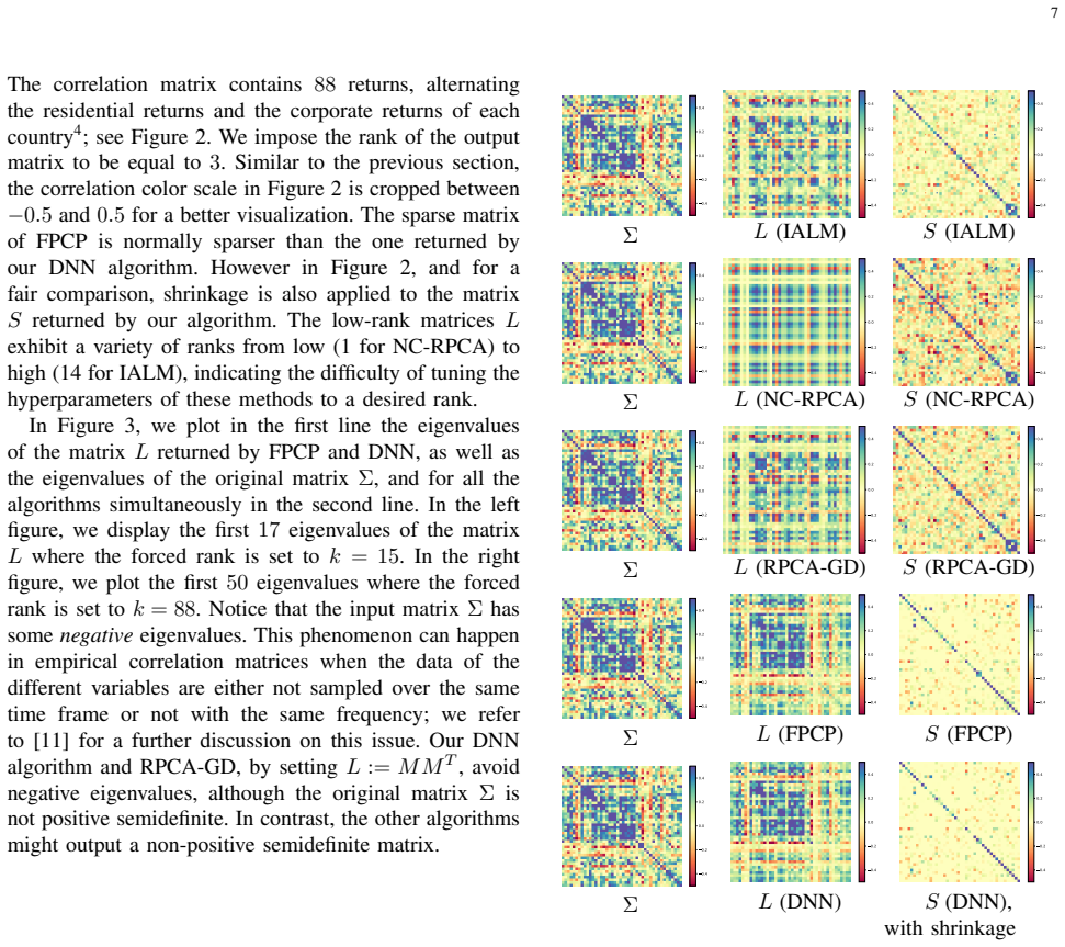
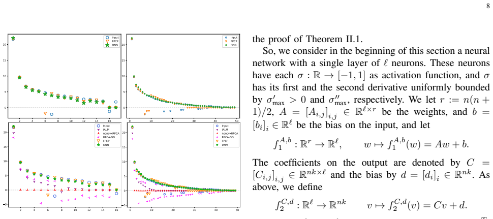
- Because $L=MM^{T}$ is always positive semidefinite, the decomposition never produces an indefinite low-rank component, even when the empirical correlation matrix has negative eigenvalues.
- Unlike nuclear-norm or PCP-style methods, the rank of $L$ is chosen in advance, so the method directly answers the portfolio problem of fixing the number of economic factors and letting the sparse part reveal residual large correlations.
- The explicit dependence of $L_m$ on the parameter bound $D$ and layer widths gives a quantitative tradeoff: smaller parameter bounds and narrower layers improve the rate constant, for fixed depth.
- The rate guarantee covers all bounded trajectories of gradient descent; the numerical experiments suggest the boundedness condition holds on realistic correlation matrices, which extends the theoretical guarantee to practice for those cases.
Reading between the lines
- An implication left implicit is that the same proof template should apply to any factorized model $L=MM^{T}$ with a Lipschitz smooth activation, not only fully connected networks; convolutional or residual parametrizations would need their own compositional Lipschitz estimates.
- The convergence guarantee concerns stationarity of the smoothed loss, not recovery of the true $(L_0,S_0)$; connecting the smoothed stationary points to exact decomposition recovery, in the style of robust PCA recovery theorems, is not addressed and may deserve separate analysis.
- A practical extension suggested by the bound is to regularize the parameters explicitly (for example, with weight decay) to keep $D$ small, since the rate constant worsens polynomially in $D$; the paper does not analyze such regularization.
- Because the loss is just a smooth approximation of $\ell^1$, the method could be extended to weighted or structured sparsity penalties by changing $\mu$ or adding a penalty term, but the convergence proof would require rechecking the second-derivative bound.
Signed reviews
Editorial analysis
A structured set of objections, weighed in public.
Referee Report
Summary. The paper proposes a method for decomposing a positive semidefinite covariance matrix Sigma into a low-rank part L = MM^T plus a sparse part S, where M is parametrized as the output of a fully connected neural network applied to the fixed input h(Sigma). The objective is a smooth approximation of ||MM^T - Sigma||_1, and the authors analyze gradient descent on the network parameters. The main theoretical result, Theorem II.1, gives an O(1/sqrt(N)) bound on the smallest gradient norm of the smoothed objective over N iterations, with a Lipschitz constant that grows polynomially in n, k, and the layer widths for fixed depth m, provided the parameter sequence remains in a fixed ball (Assumption (12)). The proof is carried out through Lemmas IV.1-IV.6, which bound the derivatives and the Lipschitz constant of the smoothed objective for single-layer and multi-layer networks. Numerical experiments on synthetic data, S&P 500 stock correlations, and real estate indices compare the method against IALM, nonconvex RPCA, RPCA-GD, and FPCP. Section III-D plots the running maximum of the parameter norm over 400 and 200 iterations on the two real datasets as empirical evidence for Assumption (12).
Significance. If the unconditional convergence claim were established, the paper would provide a first-order, SVD-free method for low-rank plus sparse covariance decomposition with a polynomial-in-dimensions complexity bound for fixed depth, and the numerical results suggest competitive empirical accuracy. The paper's main strength is the explicit and detailed computation of the Lipschitz constant of the gradient of the smoothed objective, which is a nontrivial compositional calculation; the authors also provide reproducible code and highlight the positive semidefiniteness of L by construction. However, the central theorem is conditional on an unverified boundedness assumption, the rate depends on the unknown bound D, and the convergence guarantee applies only to the smoothed surrogate, not to the original nonsmooth objective. These limitations substantially temper the advertised contribution, so the paper is best viewed as a proof-of-concept plus a worst-case smoothness analysis rather than an unconditional complexity bound.
major comments (3)
- [Section II, Theorem II.1 and Remark II.3] The convergence rate (14) is conditional on Assumption (12), sup_j ||Theta_j|| <= D. This assumption is not derived from the gradient dynamics; Remark II.3 concedes that global Lipschitzness of grad(phi) fails and that the gradient grows polynomially, of degree 4 in the single-layer case. The empirical verification in Section III-D is limited to running maxima over 400 (S&P500) and 200 (real estate) iterations on two datasets, which cannot establish an infinite-horizon bound. Moreover, the Lipschitz constant L_m in Theorem II.1 depends on D, with powers such as D^{4m+2}, so the advertised 'polynomial in dimensions' rate is in fact polynomial in dimensions and an unspecified function of D. Please either prove or enforce the boundedness of the iterates, or restate the main result as a conditional guarantee and make the D-dependence explicit in the abstract and the theorem statement.
- [Abstract and Theorem II.1] The abstract claims 'convergence rate to a local optimum', but Theorem II.1 only bounds min_{0<=j<=N} ||grad(phi)(Theta_j)|| for the smoothed surrogate phi defined in (9). Since phi is an epsilon-approximation of the nonsmooth l1 objective, a small gradient of phi does not imply stationarity of the original objective ||MM^T - Sigma||_1, let alone convergence to a local optimum of that objective. The authors should state the result as a gradient-norm bound for the smoothed surrogate and explain the relation to the original problem, for example via epsilon-stationarity in the sense of Nesterov's smoothing framework [17].
- [Remark II.2, condition (13)] The claim that a constant step-size strategy satisfies (13) with K = 1 is not justified as stated. For an L-smooth function, the standard descent lemma with step h = 1/L gives phi(Theta_j) - phi(Theta_{j+1}) >= (1/(2L))||grad(phi)(Theta_j)||^2, i.e., K = 1/2 in the notation of (13), not K = 1. Please specify the exact step-size rule that yields K = 1, or adjust the numerical constant in Remark II.2.
minor comments (4)
- [Section IV, Lemmas IV.4 and IV.5] The lemma statements write 'Theta = (A,d,C,d)', which appears to be a typo; the intended tuple is (A,b,C,d) as used in the proofs and in the single-layer formulation.
- [Section III-D and Figure 4] The running-maximum plots in Figure 4 use a very compressed y-axis scale (e.g., 36.76 to 36.81 for S&P500), which makes the visual claim of convergence difficult to assess. A plot of ||Theta_j|| itself or a logarithmic scale would be more informative.
- [Section III-A, Table II] For n = 800, the DNN row reports mean relative errors of 1.16 (1.59) for S and 0.32 (0.44) for L with large standard deviations. The text dismisses these as 'outlier instances', but the reader would benefit from a quantitative explanation of when and why these outliers occur.
- [Section II, notation around (8)] The norm ||h(Sigma)|| is used without formally defining a norm on the vectorization image of h; it is clear from context that the Euclidean norm is intended, but a brief definition would improve precision.
Circularity Check
No circularity: the convergence analysis is self-contained and conditional only on an explicit boundedness assumption; the empirically verified boundedness is not a fitted input.
full rationale
The paper's central claim is Theorem II.1: for a fixed Sigma, if the gradient-descent parameter sequence satisfies sup_j ||Theta_j|| <= D, then the gradient of the smoothed objective phi is Lipschitz on that ball with an explicit polynomial-in-dimensions constant L_m, and standard descent inequalities give the finite-time bound (14). The proof derives L_m from the compositional structure of the network (Lemmas IV.1-IV.6 and the induction in the proof of Theorem II.1) and from standard L-smooth nonconvex optimization theory; it does not use any fitted parameter, no normalization is calibrated to Sigma, and no prior result by the same authors is invoked. The only additional assumption is (12), which is explicitly stated and not derived from the dynamics; Remark II.3 even concedes that global Lipschitzness fails and that the gradient grows polynomially in the parameters. The empirical running-max checks in Section III-D support (12) on two data sets, but they are not part of the proof and do not make the theorem circular. The abstract's phrase 'convergence rate to a local optimum' overstates the gradient-norm bound in (14), but that is a correctness or interpretation gap, not circularity. No self-citation is load-bearing: the reference list contains no work by Baes, Herrera, Neufeld, or Ruyssen. Accordingly, the derivation is self-contained and the circularity score is 0.
Assumptions & free parameters
free parameters (5)
- smoothing parameter epsilon
- rank k
- network architecture (depth m, widths l_1,...,l_m, activation sigma)
- step-size sequence h_j
- boundedness constant D
assumptions (6)
- domain assumption Activation function sigma: R -> [-1,1] with uniformly bounded first and second derivatives.
- domain assumption The parameter sequence (Theta_j) stays in a bounded set (Assumption (12)).
- domain assumption The step-size strategy satisfies the sufficient decrease condition (13).
- standard math The smooth approximation mu has derivative bounded by 1 and second derivative bounded by mu''_max.
- standard math Any rank-k positive semidefinite matrix L can be factored as M M^T with M in R^{n x k}.
- standard math For L-smooth nonconvex functions, gradient descent with sufficient decrease converges to a first-order stationary point at rate O(1/N).
Cite this review
Pith. "Pith review of Low-Rank plus Sparse Decomposition of Covariance Matrices using Neural Network Parametrization." pith.science (2026). https://pith.science/paper/ICZDLQKU
@misc{pith2026190800461,
  author       = {Pith},
  title        = {Pith review of: Low-Rank plus Sparse Decomposition of Covariance Matrices using Neural Network Parametrization},
  year         = {2026},
  howpublished = {\url{https://pith.science/paper/ICZDLQKU}},
  note         = {Machine review of arXiv:1908.00461}
}
abstract
This paper revisits the problem of decomposing a positive semidefinite matrix as a sum of a matrix with a given rank plus a sparse matrix. An immediate application can be found in portfolio optimization, when the matrix to be decomposed is the covariance between the different assets in the portfolio. Our approach consists in representing the low-rank part of the solution as the product $MM^{T}$, where $M$ is a rectangular matrix of appropriate size, parametrized by the coefficients of a deep neural network. We then use a gradient descent algorithm to minimize an appropriate loss function over the parameters of the network. We deduce its convergence rate to a local optimum from the Lipschitz smoothness of our loss function. We show that the rate of convergence grows polynomially in the dimensions of the input, output, and the size of each of the hidden layers.
Figures

Figures from the paper (1 more)

Reference graph
Works this paper leans on
- [17]
-
[1]
M. Abadi, A. Agarwal, P. Barham, E. Brevdo, Z. Chen, C. Citro, G. Corrado, A. Davis, J. Dean, M. Devin, S. Ghemawat, I. Goodfellow, A. Harp, G. Irving, M. Isard, Y . Jia, R. Jozefowicz, L. Kaiser, M. Kudlur, J. Levenberg, D. Man ´e, R. Monga, S. Moore, D. Murray, C. Olah, M. Schuster, J. Shlens, B. Steiner, I. Sutskever, K. Talwar, P. Tucker, V . Vanhouck...
work page 2015
- [2]
-
[3]
T. Bouwmans, N. Aybat, and E. Zahzah. Handbook of Robust Low- Rank and Sparse Matrix Decomposition: Applications in Image and Video Processing. Chapman & Hall/CRC, 2016
work page 2016
-
[4]
T. Bouwmans, A. Sobral, S. Javed, S. Jung, and E. Zahzah. Decomposition into low-rank plus additive matrices for back- ground/foreground separation: A review for a comparative evalua- tion with a large-scale dataset. Computer Science Review, 23:1–71, 2017
work page 2017
-
[5]
T. Bouwmans, A. Sobral, and E. Zahzah. Lrslibrary: Low-rank and sparse tools for background modeling and subtraction in videos. In Robust Low-Rank and Sparse Matrix Decomposition: Applications in Image and Video Processing . CRC Press, Taylor and Francis Group, 2015
work page 2015
-
[6]
E. Cand `es, X. Li, Y . Ma, and J. Wright. Robust principal component analysis? Journal of the ACM (JACM), 58(3):11, 2011
work page 2011
-
[7]
V . Chandrasekaran, P. Parrilo, and A. Willsky. Latent variable graphical model selection via convex optimization. In 2010 48th Annual Allerton Conference on Communication, Control, and Computing (Allerton), pages 1610–1613. IEEE, 2010
work page 2010
Show all 27 references
-
[8]
Ghadimi and G
S. Ghadimi and G. Lan. Accelerated gradient methods for nonconvex nonlinear and stochastic programming. Mathematical Programming, 156(1-2):59–99, 2016
2016
-
[9]
J. He, L. Balzano, and A. Szlam. Incremental gradient on the grassmannian for online foreground and background separation in subsampled video. In 2012 IEEE Conference on Computer Vision and Pattern Recognition, pages 1568–1575, 2012
2012
-
[10]
Hestenes
M. Hestenes. Multiplier and gradient methods. Journal of Optimization Theory and Applications , 4(5):303–320, 1969
1969
-
[11]
Higham and N
N. Higham and N. Strabic. Bounds for the distance to the nearest correlation matrix. SIAM Journal on Matrix Analysis and Applications, 37(3):1088–1102, 2016
2016
-
[12]
Z. Kang, C. Peng, Q. Cheng. Robust PCA Via Nonconvex Rank Approximation. In 2015 IEEE International Conference on Data Mining, pages 211–220
2015
-
[13]
Z. Lin, M. Chen, and Y . Ma. The augmented Lagrange multi- plier method for exact recovery of corrupted low-rank matrices. arXiv:1009.5055, 2010
2010 arXiv
-
[14]
J. Liu, Y . Xu, C. Zheng, H. Kong, and Z. Lai. RPCA-based tumor classification using gene expression data. IEEE/ACM Transactions on Computational Biology and Bioinformatics , 12(4):964–970, 2015
2015
-
[15]
Lopez-Paz and L
D. Lopez-Paz and L. Sagun. Easing non-convex optimization with neural networks. https:// openreview.net/forum?id=rJXIPK1PM, 2018
2018
-
[16]
K. Min, Z. Zhang, J. Wright, and Y . Ma. Decomposing background topics from keywords by principal component pursuit. In Proceed- ings of the 19th ACM international conference on Information and knowledge management, pages 269–278. ACM, 2010
2010
-
[18]
Nesterov
Y . Nesterov. Introductory lectures on convex optimization: A basic course, volume 87. Springer Science & Business Media, 2013
2013
-
[19]
Nocedal and S
J. Nocedal and S. Wright. Numerical Optimization. Springer, 2000
2000
-
[20]
Paszke, S
A. Paszke, S. Gross, S. Chintala, G. Chanan, E. Yang, Z. DeVito, Z. Lin, A. Desmaison, L. Antiga, and A. Lerer. Automatic differentiation in Pytorch. NIPS 2017 Autodiff Workshop , 2017
2017
-
[21]
Rodriguez and B
P. Rodriguez and B. Wohlberg. Fast principal component pursuit via alternating minimization. In 2013 IEEE International Confer- ence on Image Processing , pages 69–73, 2013
2013
-
[22]
Rodriguez and B
P. Rodriguez and B. Wohlberg. Incremental principal component pursuit for video background modeling. Journal of Mathematical Imaging and Vision, 55(1):1–18, 2016
2016
-
[23]
Shahid, V
N. Shahid, V . Kalofolias, X. Bresson, M. Bronstein, and P. Van- dergheynst. Robust Principal Component Analysis on graphs. In Proceedings of the IEEE International Conference on Computer Vision, pages 2812–2820, 2015
2015
-
[24]
Shkolnik, L
A. Shkolnik, L. Goldberg, and J. Bohn. Identifying broad and narrow financial risk factors with convex optimization. SSRN 2800237, 2016
2016
-
[25]
N. Wang, T. Yao, J. Wang, and D. Yeung. A probabilistic approach to robust matrix factorization. In European Conference on Computer Vision , pages 126–139. Springer, 2012
2012
-
[26]
X. Zhou, C. Yang, and W. Yu. Moving object detection by detecting contiguous outliers in the low-rank representation. IEEE Transac- tions on pattern analysis and machine intelligence , 35(3):597–610, 2013
2013
-
[27]
X. Yi, D. Park, Y . Chen, and C. Caramanis. Fast Algorithms for Robust PCA via Gradient Descent. Advances in Neural Information Processing Systems 29 , 4152–4160, 2016
2016
Reviewed August 14, 2026 · model on record in the stance chip above.
Discussion (0). Continue with ORCID to comment.