REVIEW 3 major objections 6 minor 60 references
An implicit $ P $-multigrid flux reconstruction method for simulation of locally preconditioned unsteady Navier-Stokes equations at low Mach numbers
T0 review · 3 major / 6 minor · reviewed 2026-08-14 · deepseek-v4-flash
Pith's one-line read A P-multigrid solver for high-order flux reconstruction reaches its fastest convergence for low-Mach unsteady flows when coarse levels use polynomial degrees about half the fine degree, and it preserves high-order accuracy.
desk verdict Solid engineering paper worth a serious referee: packages known components into a working low-Mach P-multigrid solver and gives an empirically useful hierarchy rule, though the accuracy study has warts and the design rule lacks sensitivity analysis. read the letter →
The pith
A machine-rendered reading of the paper's core claim, the machinery that carries it, and where it could break.
The reading
What carries the argument
The central object is the P-multigrid V-cycle on a hierarchy of polynomial spaces, with an element Jacobi smoother performing a few relaxed updates per level. The smoother update is $q^{m+1}=q^m+\alpha_r D^{-1}F$, where $D$ is the block diagonal of the linearized pseudo-time operator and $\alpha_r=1$ in this study. The load-bearing idea is the degree-halving hierarchy: adjacent levels should differ by roughly half the finer polynomial degree, so coarse-grid corrections stay effective instead of introducing new errors. This rule is what carries the convergence acceleration.
What would settle it
Rerun the NACA0012 convergence comparisons with a different smoother configuration, for example $\alpha_r=0.5$, smoothing counts $\{10-20-40\}$, or CFL growth ratio 2.0, and check whether the fastest hierarchy shifts away from $\{P_0-P_0/2-P_0\}$ and $\{P_0-P_0/2-P_0/4-P_0/2-P_0\}$. If the ranking changes, the claimed design rule is not robust.
Extended reading notes
Core claim
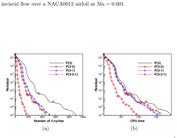
The paper establishes that an implicit P-multigrid V-cycle can be combined with locally preconditioned flux reconstruction and ESDIRK time integration without destroying high-order accuracy. Its central finding is empirical: the fastest convergence for both two-level and three-level cycles occurs when coarse polynomial degrees are near half the fine degree, specifically hierarchies close to $\{P_0-P_0/2-P_0\}$ and $\{P_0-P_0/2-P_0/4-P_0/2-P_0\}$. In the tested cases, three-level cycles beat two-level cycles, and excessive degree gaps such as $\{P_5-P_1\}$ either stall or contaminate convergence. Local preconditioning appears only in the pseudo-transient-continuation loop, so the unsteady physical time integration retains the design order of the ESDIRK method.
Load-bearing premise
The load-bearing premise is that the hierarchy ranking observed with the paper's fixed solver settings, including Jacobi relaxation $\alpha_r=1$, smoothing counts $\{5-10-20\}$, SER CFL growth ratio 1.5, smoother update intervals, and cutoff parameter $\kappa$, remains valid when those settings change; if the ranking is an artifact of the tuning, the recommended degree-halving rule collapses.
Editorial extensions
If this is right
- For a chosen fine polynomial degree, setting the coarse level near $P_0/2$ and the next near $P_0/4$ for three levels should cut both CPU time and V-cycle count relative to single-level iteration.
- Three-level cycles are preferable to two-level cycles in the tested low-Mach regime.
- Hierarchies with large adjacent degree gaps should be avoided, since they can stall convergence or cause residual oscillation.
- The combination of pseudo-time local preconditioning and P-multigrid preserves nominal high-order spatiotemporal accuracy at Ma = 0.005.
- The solver supports under-resolved transitional low-Mach wing simulations, with lift, drag, and separation/reattachment predictions consistent with prior studies.
Reading between the lines
- The degree-halving rule likely transfers to other compact high-order discretizations such as discontinuous Galerkin or spectral difference, because the mechanism is coarse-level correction effectiveness rather than the flux-reconstruction formulation; this is an inference, not tested in the paper.
- A two-grid local-mode analysis of the element Jacobi smoother with preconditioned eigenvalues could turn the empirical rule into a predictive criterion and show how the optimal ratio shifts with cell aspect ratio or Reynolds number.
- The paper's comparison of Ma = 0.1 and Ma = 0.01 wing flows leaves the cause of the difference in lift and separation bubble ambiguous; a controlled study with matched cutoff parameter and matched numerical dissipation could separate weak-compressibility effects from solver-settings effects.
- Extending the solver to Newton-Krylov with P-multigrid as a preconditioner, which the paper names as future work, is the natural test of whether the same hierarchy rule accelerates very-low-Mach nonlinear solves.
Signed reviews
Editorial analysis
A structured set of objections, weighed in public.
Referee Report
Summary. The manuscript develops an implicit P-multigrid solver for high-order flux reconstruction/correction procedure via reconstruction (FR/CPR) discretizations of the locally preconditioned unsteady compressible Navier–Stokes equations at low Mach numbers. The solver combines a FAS-type V-cycle with an element Jacobi smoother and ESDIRK temporal integration, with local preconditioning applied only in the pseudo-time continuation to preserve time accuracy. Accuracy is verified on an isentropic vortex at Ma=0.005, the influence of polynomial-degree hierarchies is studied on 2D inviscid and viscous NACA0012 flows and a 3D sphere flow at Ma=0.001, and the solver is applied to an under-resolved transitional SD7003 wing at Re=60000 and Ma=0.1/0.01. The authors recommend hierarchies close to {P0-P0/2-P0} for two-level and {P0-P0/2-P0/4-P0/2-P0} for three-level V-cycles as giving the best convergence acceleration.
Significance. If the empirical hierarchy rule is robust, the paper offers a practical acceleration strategy for high-order low-Mach FR/CPR solvers, addressing a known stiffness problem in a way that is directly useful for coarse-resolution turbulence simulation. The manuscript is clearly organized, provides a complete algorithmic description, and includes a challenging 3D application with quantitative comparisons to previous experimental and numerical results. The central claims are conditional, however: the order-of-accuracy verification is incomplete for density and pressure at the finest resolutions, and the hierarchy recommendation is obtained with a fixed set of solver parameters and without work-per-cycle normalization, so its generality is not yet established.
major comments (3)
- [§4.1, Tables 1 and 2] The order-of-accuracy verification does not fully support the claim of verified high-order spatiotemporal accuracy. In Table 1, ESDIRK4 shows order drops to 0.79 for density and 1.39 for pressure at the finest time step, while velocity retains order 4.00. In Table 2, the P3 and P4 FR schemes similarly show density and pressure order collapse at the finest grid (e.g., P3 density order 0.49, P4 density order 0.02), while velocity continues to converge. The authors attribute these reductions to "the accuracy limit of the solver," but do not identify this limit or explain why velocity is unaffected. Because the abstract and conclusions state that high-order spatiotemporal accuracy is verified, this inconsistency must be addressed, either by tightening the pseudo-time tolerance, analyzing the effect of the 1e-4 tolerance on each variable, or rephrasing the accuracy claim.
- [§4.2, Figures 4–6, 8–10, 12–13] The central hierarchy recommendation is based on a fixed set of solver parameters (I{5-10-20}, alpha_r=1, SER growth ratio 1.5, CFLinit=1e2, CFLmax=1e5, kappa=1) with no sensitivity study. It is therefore unclear whether the observed ranking of hierarchies, e.g., P{4-2} over P{4-1} or P{5-3-1} over P{5-4-1}, persists for other smoothing schedules, relaxation parameters, or CFL update strategies. A sensitivity study or a two-grid analysis is needed to show that the recommended rule "polynomial degree difference close to half of the finer degree" is a property of the multigrid correction rather than an artifact of the chosen parameters.
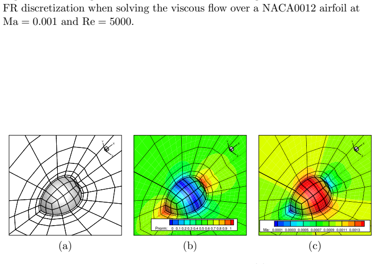
- [§4.2, CPU-time and V-cycle comparisons] The comparison across hierarchies is not normalized for the cost of smoothing sweeps at different polynomial degrees. All two-level cases use I{5-10} and all three-level cases use I{5-10-20}, so a V-cycle for P{5-4-1} performs the same number of sweeps as one for P{5-2-1}, but the sweeps at P4 are much more expensive than those at P2 or P1. The residual-versus-V-cycle plots partially mitigate this, but the CPU-time comparisons would be more interpretable if the paper reported the cost per smoothing sweep at each degree and the total work per V-cycle for each hierarchy. Without this information, the reader cannot separate the benefit of coarse-grid correction from the effect of concentrating smoothing effort on cheaper lower-degree spaces.
minor comments (6)
- [§2.3, Eq. (15)] There is a typo: "The ensure conservation" should read "To ensure conservation."
- [§4.2.1] The statement that P{3-2} and P{3-1} have "almost the same computational cost" is vague, since P{3-1} uses a cheaper coarse level; please clarify whether the similar cost arises because P{3-1} requires more V-cycles, which is not apparent from the figures.
- [§4.3] The choice of the global cutoff parameter kappa=2.5 for Ma=0.01, while kappa=1.0 for Ma=0.1, is stated without justification; a brief explanation of how this cutoff value was selected would improve reproducibility.
- [Figure 18] The axis labels contain typos: "Peudo iteration m" and "resisual" should be "Pseudo iteration m" and "residual."
- [§3] The restriction and prolongation operators (PP0_P1 and IP1_P0) are not defined; specifying whether they are L2 projections or interpolation operators would make the algorithm fully reproducible.
- [§4.2.1] The convergence histories in Figures 4–6 are shown down to residual 1e-9, but the stopping criterion or target tolerance for the steady-state cases is not stated; please include it.
Circularity Check
No significant circularity: the central claims are supported by in-paper numerical experiments and external benchmarks, not by self-citation or by fitted inputs renamed as predictions.
full rationale
The paper's central claims are: (1) the P-multigrid solver preserves high-order spatiotemporal accuracy; (2) polynomial hierarchies near {P0-P0/2-P0} or {P0-P0/2-P0/4-P0/2-P0} give the best convergence acceleration; and (3) coarse SD7003 simulations agree with prior experimental and numerical data. Claim (1) is validated against the analytic isentropic vortex in Section 4.1, Tables 1 and 2, so it does not reduce to an input or fitted parameter. Claim (2) is an empirical comparison made in Sections 4.2.1-4.2.3 using convergence histories for many fixed hierarchies; the paper explicitly says 'our numerical experiments consistently suggest' the hierarchy rule, and the evidence is the in-paper residual and CPU-time histories. The conference paper [52] is cited only as prior preliminary work, not as the load-bearing justification for the hierarchy recommendation. Claim (3) is checked against experimental results (Selig et al.) and independent numerical studies (Vermeire et al., Beck et al., Galbraith and Visbal), so it is externally falsifiable. The self-citations ([8], [16], [26], [52]) are contextual or preliminary and do not carry the central derivation. The fixed smoothing schedules and the cutoff parameter kappa are hand-tuned, and no sensitivity or work-normalization study is provided, but that is a robustness and cost-accounting concern rather than evidence that any prediction reduces to its own inputs by construction. No self-definitional step, fitted quantity renamed as prediction, or author-supplied uniqueness theorem was found.
Assumptions & free parameters
free parameters (6)
- global cutoff parameter kappa =
1.0 for most cases; 2.5 for SD7003 at Ma=0.01
- CFLinit and CFLmax =
1e2 and 1e5 for airfoil/sphere studies; for the vortex, Delta_tau_init=0.01 and Delta_tau_max=10; for SD7003…
- Smoothing iteration counts I{n0-n1-n2} =
I{5-10-20}, I{5-10}, I{10}, I{20-20-40}, I{5-5-10}, I{10-10-16}
- SER growth ratio =
1.5
- Smoother update interval =
every 10 pseudo iterations; every 20 for Ma=0.01 SD7003
- Relaxation parameter alpha_r =
1.0
assumptions (7)
- domain assumption The Weiss-Smith local preconditioning matrix Gamma (Eq. 9) with reference velocity Ur = epsilon c balances characteristic speeds and preserves the steady state of the unpreconditioned equations.
- standard math The FR/CPR differential form (Eq. 20) with correction field delta_e is equivalent to the weak form, and tensor-product correction polynomials are valid on quadrilaterals and hexahedra.
- domain assumption The approximate Riemann solver of Ref. [7] (Eq. 21) provides a stable common inviscid flux at low Mach numbers.
- domain assumption The BR2 viscous flux treatment from Ref. [55] yields stable and consistent viscous common fluxes.
- domain assumption The dual-time stepping fixed point of Eq. (27) equals the ESDIRK stage solution F(q)=0, so preconditioning only in pseudo-time preserves physical-time accuracy.
- ad hoc to paper The element Jacobi smoother (Eq. 30) with block-diagonal D is a convergent smoother for the P-multigrid V-cycle on the tested meshes.
- ad hoc to paper The FAS P-multigrid correction algorithm (Section 3) converges for low-Mach preconditioned systems when the hierarchy satisfies the recommended rule.
Cite this review
Pith. "Pith review of An implicit $ P $-multigrid flux reconstruction method for simulation of locally preconditioned unsteady Navier-Stokes equations at low Mach numbers." pith.science (2026). https://pith.science/paper/IERUCZFV
@misc{pith2026190803972,
  author       = {Pith},
  title        = {Pith review of: An implicit $ P $-multigrid flux reconstruction method for simulation of locally preconditioned unsteady Navier-Stokes equations at low Mach numbers},
  year         = {2026},
  howpublished = {\url{https://pith.science/paper/IERUCZFV}},
  note         = {Machine review of arXiv:1908.03972}
}
abstract
We develop a $ P $-multigrid solver to simulate locally preconditioned unsteady compressible Navier-Stokes equations at low Mach numbers with implicit high-order methods. Specifically, the high-order flux reconstruction/correction procedure via reconstruction (FR/CPR) method is employed for spatial discretization and the high-order time integration is conducted by means of the explicit first stage, singly diagonally implicit Runge-Kutta (ESDIRK) method. Local preconditioning is used to alleviate the stiffness of the compressible Navier-Stokes equations at low Mach numbers and is only conducted in pseudo transient continuation to ensure the high-order accuracy of ESDIRK methods. We employ the element Jacobi smoother to update the solutions at different $ P $-levels in the $ P $-multigrid solver. High-order spatiotemporal accuracy of the new solver for low-Mach-number flow simulation is verified with the isentropic vortex propagation when the Mach (Ma) number of the free stream is 0.005. The impact of the hierarchy of polynomial degrees on the convergence speed of the $ P $-multigrid method is studied via several numerical experiments, including two dimensional (2D) inviscid and viscous flows over a NACA0012 airfoil at $\text{Ma} = 0.001$, and a three dimensional (3D) inviscid flow over a sphere at $\text{Ma} = 0.001$. The $ P $-multigrid solver is then applied to coarse resolution simulation of the transitional flows over an SD7003 wing at $ 8^\circ $ angle of attack when the Reynolds number is 60000 and the Mach number is 0.1 or 0.01.
Figures


Figures from the paper (16 more)




Reference graph
Works this paper leans on
-
[1]
On the accuracy of high-order dis- cretizations for underresolved turbulence simulations,
G. J. Gassner and A. D. Beck, “On the accuracy of high-order dis- cretizations for underresolved turbulence simulations,” Theoretical and Computational Fluid Dynamics , vol. 27, pp. 221–237, 2013
work page 2013
-
[2]
R. C. Moura, S. J. Sherwin, and J. Peir´ o, “Linear dispersion–diffusion analysis and its application to under-resolved turbulence simulations using discontinuous Galerkin spectral/hp methods,” Journal of Com- putational Physics, vol. 298, pp. 695–710, 2015
work page 2015
-
[3]
F. Bassi, L. Botti, A. Colombo, A. Crivellini, A. Ghidoni, and F. Massa, “On the development of an implicit high-order discontinuous Galerkin method for DNS and implicit LES of turbulent flows,” European Jour- nal of Mechanics-B/Fluids , vol. 55, pp. 367–379, 2016
work page 2016
-
[4]
Towards industrial large eddy simulation using the FR/CPR method,
Z. Wang, Y. Li, F. Jia, G. Laskowski, J. Kopriva, U. Paliath, and R. Bhaskaran, “Towards industrial large eddy simulation using the FR/CPR method,” Computer & Fluids , vol. 156, pp. 579–589, 2017
work page 2017
-
[5]
Preconditioned methods for solving the incompressible and low speed compressible equations,
E. Turkel, “Preconditioned methods for solving the incompressible and low speed compressible equations,” Journal of computational physics , vol. 72, no. 2, pp. 277–298, 1987
work page 1987
-
[6]
Preconditioning and the limit to the incompressible flow equations,
E. Turkel, A. Fiterman, and B. Van Leer, “Preconditioning and the limit to the incompressible flow equations,” tech. rep., Institute for Computer Applications in Science and Engineering Hampton VA, 1993
work page 1993
-
[7]
Preconditioning applied to variable and constant density Flows,
J. M. Weiss and W. A. Smith, “Preconditioning applied to variable and constant density Flows,” AIAA Journal, vol. 33, no. 11, 1995
work page 1995
-
[8]
L. Wang and M. Yu, “An Implicit High-Order Preconditioned Flux Re- construction Method for Low-Mach-Number Flow Simulation with Dy- namic Meshes,” International Journal for Numerical Methods in Fluids,
Show all 60 references
-
[9]
A flux reconstruction approach to high-order schemes including discontinuous Galerkin methods,
H. T. Huynh, “A flux reconstruction approach to high-order schemes including discontinuous Galerkin methods,” in the 18th AIAA Compu- tational Fluid Dynamics Conference , (Miami, FL), 2007. AIAA-2007- 4079
2007
-
[10]
A reconstruction approach to high-order schemes includ- ing discontinuous Galerkin methods for diffusion,
H. T. Huynh, “A reconstruction approach to high-order schemes includ- ing discontinuous Galerkin methods for diffusion,” in the 47th AIAA Aerospace Sciences Meeting including The New Horizons Forum and Aerospace, (Orlando, FL), 2009. AIAA-2009-403. 27
2009
-
[11]
A unifying lifting collocation penalty formulation including the discontinuous Galerkin, spectral vol- ume/difference methods for conservation laws on mixed grids,
Z. J. Wang and H. Y. Gao, “A unifying lifting collocation penalty formulation including the discontinuous Galerkin, spectral vol- ume/difference methods for conservation laws on mixed grids,” Journal of Computational Physics , vol. 228, pp. 8161–8186, 2009
2009
-
[12]
A new class of high- order energy stable flux reconstruction schemes,
P. E. Vincent, P. Castonguay and A. Jameson, “A new class of high- order energy stable flux reconstruction schemes,” Journal of Scientific Computing, vol. 47, pp. 50–72, 2011
2011
-
[13]
Implicit time integration schemes for the unsteady compressible Navier–Stokes equations: laminar flow,
H. Bijl, M. H. Carpenter, V. N. Vatsa, and C. A. Kennedy, “Implicit time integration schemes for the unsteady compressible Navier–Stokes equations: laminar flow,” Journal of Computational Physics , vol. 179, no. 1, pp. 313–329, 2002
2002
-
[14]
Diagonally Implicit Runge-Kutta Methods for Ordinary Differential Equations. A Review,
C. A. Kennedy and M. H. Carpenter, “Diagonally Implicit Runge-Kutta Methods for Ordinary Differential Equations. A Review,” Tech. Rep. NASA/TM–2016–219173, NASA
2016
-
[15]
Linearly implicit Rosenbrock-type Runge–Kutta schemes applied to the Discon- tinuous Galerkin solution of compressible and incompressible unsteady flows,
F. Bassi, L. Botti, A. Colombo, A. Ghidoni, and F. Massa, “Linearly implicit Rosenbrock-type Runge–Kutta schemes applied to the Discon- tinuous Galerkin solution of compressible and incompressible unsteady flows,” Computers & Fluids , vol. 118, pp. 305–320, 2015
2015
-
[16]
A comparative study of implicit Jacobian-free Rosenbrock-Wanner, ESDIRK and BDF methods for unsteady flow simulation with high-order flux reconstruction formulations,
L. Wang and M. Yu, “A comparative study of implicit Jacobian-free Rosenbrock-Wanner, ESDIRK and BDF methods for unsteady flow simulation with high-order flux reconstruction formulations,” arXiv preprint arXiv:1904.04825, 2019
1904 arXiv
-
[17]
Numerical solution of the Euler equations with a multiorder discontinuous finite element method,
F. Bassi and S. Rebay, “Numerical solution of the Euler equations with a multiorder discontinuous finite element method,” in Computational Fluid Dynamics 2002 , pp. 199–204, Springer, 2003
2002
-
[18]
p-Multigrid solution of high-order discontinuous Galerkin discretizations of the com- pressible Navier–Stokes equations,
K. J. Fidkowski, T. A. Oliver, J. Lu, and D. L. Darmofal, “p-Multigrid solution of high-order discontinuous Galerkin discretizations of the com- pressible Navier–Stokes equations,” Journal of Computational Physics , vol. 207, no. 1, pp. 92–113, 2005
2005
-
[19]
High-order discontinuous galerkin methods using an hp-multigrid approach,
C. R. Nastase and D. J. Mavriplis, “High-order discontinuous galerkin methods using an hp-multigrid approach,” Journal of Computational Physics, vol. 213, no. 1, pp. 330–357, 2006
2006
-
[20]
A p-multigrid discontinuous Galerkin method for the Euler equations on unstructured grids,
H. Luo, J. D. Baum, and R. L¨ ohner, “A p-multigrid discontinuous Galerkin method for the Euler equations on unstructured grids,” Jour- nal of Computational Physics , vol. 211, no. 2, pp. 767–783, 2006
2006
-
[21]
A p-multigrid spectral difference method with explicit and implicit smoothers on unstructured triangular grids,
C. Liang, R. Kannan, and Z. Wang, “A p-multigrid spectral difference method with explicit and implicit smoothers on unstructured triangular grids,” Computers & fluids , vol. 38, no. 2, pp. 254–265, 2009. 28
2009
-
[22]
A high-order flux reconstruction/correction pro- cedure via reconstruction formulation for unsteady incompressible flow on unstructured moving grids,
M. Yu and L. Wang, “A high-order flux reconstruction/correction pro- cedure via reconstruction formulation for unsteady incompressible flow on unstructured moving grids,” Computers & Fluids, vol. 139, pp. 161– 173, 2016
2016
-
[23]
On the efficiency of a matrix-free linearly implicit time integration strategy for high-order dis- continuous Galerkin solutions of incompressible turbulent flows,
M. Franciolini, A. Crivellini, and A. Nigro, “On the efficiency of a matrix-free linearly implicit time integration strategy for high-order dis- continuous Galerkin solutions of incompressible turbulent flows,” Com- puters & Fluids , vol. 159, pp. 276–294, 2017
2017
-
[24]
A high- order cross-platform incompressible Navier–Stokes solver via artificial compressibility with application to a turbulent jet,
N. Loppi, F. D. Witherden, A. Jameson, and P. E. Vincent, “A high- order cross-platform incompressible Navier–Stokes solver via artificial compressibility with application to a turbulent jet,” Computer Physics Communications, vol. 233, pp. 193–205, 2018
2018
-
[25]
A simplified formulation of the flux reconstruction method,
J. Romero, K. Asthana and A. Jameson, “A simplified formulation of the flux reconstruction method,” Journal of Scientific Computing , vol. 67, pp. 351–372, 2016
2016
-
[26]
Compact direct flux reconstruction for conser- vation laws,
L. Wang and M. Yu, “Compact direct flux reconstruction for conser- vation laws,” Journal of Scientific Computing , vol. 75, pp. 253–275, 2018
2018
-
[27]
Discontinuous Galerkin via Interpolation: The Direct Flux Reconstruction Method,
H. T. Huynh, “Discontinuous Galerkin via Interpolation: The Direct Flux Reconstruction Method,” in AIAA Aviation 2019 Forum, (Dallas, Texas), 2019. AIAA 2005-3064
2019
-
[28]
TVB Runge-Kutta local projection dis- continuous Galerkin finite element method for conservation laws. II. General framework,
B. Cockburn and C.-W. Shu, “TVB Runge-Kutta local projection dis- continuous Galerkin finite element method for conservation laws. II. General framework,” Mathematics of computation , vol. 52, no. 186, pp. 411–435, 1989
1989
-
[29]
A high-order accurate discontinuus finite el- ement method for the numerical solution of the compressible Navier– Stokes equations,
F. Bassi and S. Rebay, “A high-order accurate discontinuus finite el- ement method for the numerical solution of the compressible Navier– Stokes equations,” Journal of computational physics , vol. 131, no. 2, pp. 267–279, 1997
1997
-
[30]
Discontinuous Galerkin for diffusion,
B. van Leer and S. Nomura, “Discontinuous Galerkin for diffusion,” in the 17th AIAA Computational Fluid Dynamics Conference , (Toronto, Ontario, Canada), 2005. AIAA-2005-5108
2005
-
[31]
Implicit solution of the unsteady Eu- ler equations for high-order accurate discontinuous Galerkin discretiza- tions,
L. Wang and D. J. Mavriplis, “Implicit solution of the unsteady Eu- ler equations for high-order accurate discontinuous Galerkin discretiza- tions,” Journal of Computational Physics , vol. 225, no. 2, pp. 1994– 2015, 2007. 29
1994
-
[32]
J. S. Hesthaven and T. Warburton, Nodal Discontinuous Galerkin Methods: Algorithms, Analysis, and Applications . New York: Springer- Verlag, 2008
2008
-
[33]
Spectral (Finite) Volume Method for Conservation Laws on Unstructured Grids. Basic Formulation: Basic Formulation,
Z. J. Wang, “Spectral (Finite) Volume Method for Conservation Laws on Unstructured Grids. Basic Formulation: Basic Formulation,” Jour- nal of Computational Physics , vol. 178, no. 1, pp. 210–251, 2002
2002
-
[34]
A Conservative Staggered-Grid Cheby- shev Multidomain Method for Compressible Flows,
D. A. Kopriva and J. H. Kolias, “A Conservative Staggered-Grid Cheby- shev Multidomain Method for Compressible Flows,” Journal of Com- putational Physics, vol. 125, no. 1, pp. 244–261, 2002
2002
-
[35]
Spectral difference method for unstructured grids I: basic formulation,
Y. Liu, M. Vinokur, and Z. J. Wang, “Spectral difference method for unstructured grids I: basic formulation,” Journal of Computational Physics, vol. 216, no. 2, pp. 780–801, 2006
2006
-
[36]
High-order methods for computational fluid dynamics: A brief review of compact differen- tial formulations on unstructured grids,
H. T. Huynh, Z. J. Wang, and P. E. Vincent, “High-order methods for computational fluid dynamics: A brief review of compact differen- tial formulations on unstructured grids,” Computers & fluids , vol. 98, pp. 209–220, 2014
2014
-
[37]
Strong stability-preserving high-order time discretization methods,
S. Gottlieb, C.-W. Shu, and E. Tadmor, “Strong stability-preserving high-order time discretization methods,” SIAM review, vol. 43, no. 1, pp. 89–112, 2001
2001
-
[38]
Jacobian-free Newton–Krylov methods: a survey of approaches and applications,
D. A. Knoll and D. E. Keyes, “Jacobian-free Newton–Krylov methods: a survey of approaches and applications,” Journal of Computational Physics, vol. 193, no. 2, pp. 357–397, 2004
2004
-
[39]
Newton-GMRES preconditioning for dis- continuous Galerkin discretizations of the Navier–Stokes equations,
P.-O. Persson and J. Peraire, “Newton-GMRES preconditioning for dis- continuous Galerkin discretizations of the Navier–Stokes equations,” SIAM Journal on Scientific Computing , vol. 30, no. 6, pp. 2709–2733, 2008
2008
-
[40]
On the computation of compressible turbulent flows on unstructured grids,
H. Luo, D. Sharov, J. D. Baum, and R. Loehner, “On the computation of compressible turbulent flows on unstructured grids,” International Journal of Computational Fluid Dynamics , vol. 14, no. 4, pp. 253–270, 2001
2001
-
[41]
An implicit matrix-free discontinuous Galerkin solver for viscous and turbulent aerodynamic simulations,
A. Crivellini and F. Bassi, “An implicit matrix-free discontinuous Galerkin solver for viscous and turbulent aerodynamic simulations,” Computers & fluids , vol. 50, no. 1, pp. 81–93, 2011
2011
-
[42]
Efficient time inte- gration for discontinuous Galerkin methods for the unsteady 3d Navier- Stokes equations,
P. Birken, G. Gassner, M. Haas, and C.-D. Munz, “Efficient time inte- gration for discontinuous Galerkin methods for the unsteady 3d Navier- Stokes equations,” in European Congress on Computational Methods and Applied Sciences and Engineering (ECCOMAS 2012), number Ec- comas, 2012. 30
2012
-
[43]
Preconditioning for modal discontinuous Galerkin methods for unsteady 3D Navier– Stokes equations,
P. Birken, G. Gassner, M. Haas, and C.-D. Munz, “Preconditioning for modal discontinuous Galerkin methods for unsteady 3D Navier– Stokes equations,” Journal of Computational Physics , vol. 240, pp. 20– 35, 2013
2013
-
[44]
A numerical investigation of matrix-free implicit time- stepping methods for large CFD simulations,
A. Sarshar, P. Tranquilli, B. Pickering, A. McCall, C. J. Roy, and A. Sandu, “A numerical investigation of matrix-free implicit time- stepping methods for large CFD simulations,” Computers & Fluids , vol. 159, pp. 53–63, 2017
2017
-
[45]
Solution of the Euler equations for two dimensional tran- sonic flow by a multigrid method,
A. Jameson, “Solution of the Euler equations for two dimensional tran- sonic flow by a multigrid method,”Appl. Math. Comput, vol. 13, no. 3-4, pp. 327–355, 1983
1983
-
[46]
Multigrid solution of the Navier- Stokes equations on triangular meshes,
D. J. Mavriplis and A. Jameson, “Multigrid solution of the Navier- Stokes equations on triangular meshes,” AIAA journal, vol. 28, no. 8, pp. 1415–1425, 1990
1990
-
[47]
Multigrid solution of the 3-D compressible Euler equations on unstructured tetrahedral grids,
J. Peraire, J. Peiro, and K. Morgan, “Multigrid solution of the 3-D compressible Euler equations on unstructured tetrahedral grids,” Inter- national Journal for Numerical Methods in Engineering , vol. 36, no. 6, pp. 1029–1044, 1993
1993
-
[48]
A Multigrid Preconditioned Newton– Krylov Method,
D. A. Knoll and W. J. Rider, “A Multigrid Preconditioned Newton– Krylov Method,” SIAM Journal on Scientific Computing, vol. 21, no. 2, pp. 691–710, 1999
1999
-
[49]
Analysis of“p
B. Helenbrook, D. Mavriplis, and H. Atkins, “Analysis of“p”-Multigrid for Continuous and Discontinuous Finite Element Discretizations,” in 16th AIAA Computational Fluid Dynamics Conference , p. 3989, 2003
2003
-
[50]
Multigrid solver algorithms for dg methods and applications to aerodynamic flows,
M. Wallraff, R. Hartmann, and T. Leicht, “Multigrid solver algorithms for dg methods and applications to aerodynamic flows,” inIDIHOM: In- dustrialization of High-Order Methods-A Top-Down Approach, pp. 153– 178, Springer, 2015
2015
-
[51]
P-multigrid precondi- tioners applied to high-order dg and hdg discretizations,
M. Franciolini, K. Fidkowski, and A. Crivellini, “P-multigrid precondi- tioners applied to high-order dg and hdg discretizations,” in 7th Euro- pean Conference on Computational Fluid Dynamics, Glasgow, Scotland, vol. 50, pp. 2–5, 2018
2018
-
[52]
A p-multigrid flux reconstruction method for the steady Navier-Stokes equations,
L. Wang and M. L. Yu, “A p-multigrid flux reconstruction method for the steady Navier-Stokes equations,” in AIAA Aviation 2019 Forum , (Dallas, TX), 2019. AIAA 2019-3061
2019
-
[53]
On the connection between the correction and weighting functions in the correction procedure via reconstruction method,
M. Yu and Z. J. Wang, “On the connection between the correction and weighting functions in the correction procedure via reconstruction method,” Journal of Scientific Computing , vol. 54, pp. 227–244, 2013. 31
2013
-
[54]
Energy Stable Flux Reconstruction Schemes for Advection- Diffusion Problems on Triangles,
Williams, D. M. and Castonguay, P. and Vincent, P. E. and Jame- son, A., “Energy Stable Flux Reconstruction Schemes for Advection- Diffusion Problems on Triangles,” Journal of Computational Physics , vol. 250, pp. 53–76, 2013
2013
-
[55]
Discontinuous Galerkin solution of the Reynolds-averaged Navier–Stokes andk–ω tur- bulence model equations,
F. Bassi, A. Crivellini, S. Rebay, and M. Savini, “Discontinuous Galerkin solution of the Reynolds-averaged Navier–Stokes andk–ω tur- bulence model equations,” Computer & Fluids , vol. 34, pp. 507–540, 2005
2005
-
[56]
Experiments with implicit upwind methods for the Euler equations,
W. A. Mulder and B. Van Leer, “Experiments with implicit upwind methods for the Euler equations,” Journal of Computational Physics , vol. 59, no. 2, pp. 232–246, 1985
1985
-
[57]
M. S. Selig, Summary of low speed airfoil data Vol. 1 . SoarTech Publi- cations, 1995
1995
-
[58]
On the utility of GPU accelerated high-order methods for unsteady flow simulations: A comparison with industry-standard tools,
B. C. Vermeire, F. D. Witherden, and P. E. Vincent, “On the utility of GPU accelerated high-order methods for unsteady flow simulations: A comparison with industry-standard tools,” Journal of Computational Physics, vol. 334, pp. 497–521, 2017
2017
-
[59]
High-order discontinuous Galerkin spectral element methods for transitional and turbulent flow simulations,
A. D. Beck, T. Bolemann, D. Flad, H. Frank, G. J. Gassner, F. Hin- denlang, and C.-D. Munz, “High-order discontinuous Galerkin spectral element methods for transitional and turbulent flow simulations,” In- ternational Journal for Numerical Methods in Fluids , vol. 76, no. 8, pp...
2014
-
[60]
Implicit large eddy simulation of low reynolds number flow past the sd7003 airfoil,
M. Galbraith and M. Visbal, “Implicit large eddy simulation of low reynolds number flow past the sd7003 airfoil,” in 46th AIAA Aerospace Sciences Meeting and Exhibit , p. 225, 2008. 32
2008
Reviewed August 14, 2026 · model on record in the stance chip above.
Discussion (0). Continue with ORCID to comment.