REVIEW 4 major objections 3 minor 14 references
Observable Estimation in the Absence of Classical Verification
T0 review · 4 major / 3 minor · reviewed 2026-08-01 · deepseek-v4-flash
Pith's one-line read This paper claims that quantum estimates of observables can be judged credible without any classical ground truth, by testing the noise assumptions behind error mitigation on the target circuit itself.
desk verdict Real validation framework for unbenchmarkable quantum estimates; the most-credible claim is conditional but honestly argued and worth a serious referee. read the letter →
The pith
A machine-rendered reading of the paper's core claim, the machinery that carries it, and where it could break.
The reading
What carries the argument
The central object is the operator Loschmidt echo Sδ = 2^{-n} Tr(U†OU Vδ† U†OU Vδ), an overlap between an evolved observable and its perturbed echo; unlike the state echo, it decays only polynomially with perturbation support, so it survives hardware noise. The first mechanism is global rescaling: noise is assumed to attenuate the echo by a factor α independent of probe strength δ, estimated from the δ=0 signal and divided out. The second is probabilistic error cancellation with a sparse Pauli–Lindblad noise model, which replaces the assumption with a validated noise model and provides confidence intervals.
What would settle it
Measure the L=6 echo at two probe strengths (δ=0 and δ=0.3) while deliberately adding a known coherent error common to both, such as a fixed single-qubit over-rotation in every CZ layer. If the ratio of the two decay factors changes as the injected error grows, the attenuation factor is δ-dependent and the rescaled curve is biased.
Extended reading notes
Core claim
Central claim: for the 56-qubit operator Loschmidt echo at depth L=6, the globally rescaled quantum measurement is the most credible estimate among all methods tested. Without any exact classical benchmark, the authors show the rescaling tracks converged classical results at shallow depths, is stable under deliberate noise changes (gate duration, a second processor, synthetic noise), and obeys the assumed δ-independence of the noise attenuation factor. A separate arm, probabilistic error cancellation with a validated sparse Pauli–Lindblad noise model, adds error bounds and agrees with classical results where available. Trust follows from noise-model validation, not classical agreement.
Load-bearing premise
The rescaling estimate rests on the assumption that hardware noise attenuates the echo signal by a factor that does not depend on the probe strength δ; this is tested directly only at shallow depths, while at L=6 it is inferred from cross-device consistency.
Editorial extensions
If this is right
- Quantum estimates can be declared credible in regimes where all classical heuristics disagree, provided they pass noise-manipulation consistency tests on the target circuit.
- The global rescaling estimate costs only one extra measurement at δ=0 and needs no classical simulation, making it a practical validation tool for echo-type signals.
- PEC-based error bounds shift the burden of proof from reproducing a classical answer to characterizing the hardware noise accurately.
- The operator Loschmidt echo provides an experimentally accessible probe of operator spreading and backflow at scales where state Loschmidt echoes are unmeasurable.
- Classical heuristic developers can use the same validation hierarchy, and well-characterized quantum experiments can in turn benchmark novel classical approximations.
Reading between the lines
- The validation hierarchy generalizes beyond this observable: any heuristic error-mitigation method could be trusted by showing stability under controlled noise manipulation, even when no classical check exists.
- If δ-independent attenuation continues to hold at deeper circuits, global rescaling may combine with PEC to produce bounded estimates for a wide class of echo observables, not just the operator Loschmidt echo.
- A sharp test of the framework would be to apply it to an observable with a known exact value at large depth, such as a conserved quantity, and check whether the stability tests still predict credibility.
- The paper's logic inverts the usual verification arrow: once quantum estimates are trusted, they become references for classical simulation development, potentially accelerating progress on both sides.
Editorial analysis
A structured set of objections, weighed in public.
Referee Report
Summary. The paper proposes a validation framework for quantum-computed observables in regimes where no reliable classical benchmark exists. It applies this framework to a 56-qubit semi-scrambling Floquet circuit, measuring an operator Loschmidt echo (OLE) and estimating the signal via a global-rescaling error-mitigation heuristic. The quantum estimate is compared with TN-BP, PP-MC, MPS, TTN, quarter-out Pauli propagation, and a full-scrambling analytical value; the authors claim that at depth L=6 the quantum experiment is the most credible of the methods tested, based on shallow-depth agreement, noise-manipulation stability, and cross-device consistency. A second method, PEC with a validated sparse Pauli-Lindblad noise model, provides error-bounded estimates at L=2 and L=4, with extensions to larger depth only projected.
Significance. If the framework is accepted, it offers a genuinely useful alternative to the circular standard of validating a quantum computation by agreement with a classical calculation. The paper's strengths include an honest and unusually thorough multi-method classical benchmarking campaign, direct tests of the rescaling assumption at shallow depth, cross-device and synthetic-noise manipulations, a meticulous PEC noise-model validation suite (Pauli-ness, sparsity, Markovianity, Cliffordization), and the introduction of the OLE as a hardware-accessible probe of operator dynamics. The manuscript is also commendably candid about the failures and non-convergence of the classical heuristics it considers. However, the strongest claim — that the L=6 quantum estimate is the most credible method — rests on an assumption whose direct verification is limited to depths L≤4.
major comments (4)
- [Building trust in the quantum estimate, Fig. 2(d)] The L=6 cross-device consistency check is a relative test. It compares decay factors across noise profiles after referencing to ibm_boston, and can therefore only test whether alpha_delta/alpha_0 is the same for the different profiles; it cannot detect a delta-dependent attenuation that is common to all profiles. A concrete mechanism exists: the perturbation V_delta is implemented as RX(delta) gates on 35 qubits, while at delta=0 these gates are absent. Errors in those RX gates (including coherent or angle-dependent errors) enter S~_delta but not S~_0, so alpha_delta/alpha_0 could deviate from 1 by a common factor across all devices and synthetic noise settings. The direct delta-independence test in Fig. 2(b) is performed only at L=3,4. Thus the headline L=6 curve in Fig. 1(e) may carry an unquantified systematic bias, and the statement that the quantum estimate is 'the most credible of
- [Building trust in the quantum estimate, Fig. 2(c)] The collapse of the globally rescaled signals under hardware changes and synthetic noise injections is evidence that the attenuation factor is stable with respect to the noise profile, but it is not evidence that the attenuation factor is delta-independent. The text says these manipulations 'provide evidence that the global rescaling captures the dominant effect of noise on the target circuits'; this conflates profile-independence with delta-independence. The caption and main text should distinguish the two, since the delta-independence of alpha is the assumption needed for the global-rescaling estimator S_delta ≈ S~_delta / S~_0.
- [Towards estimation with error bounds, Figs. 3(f)-(g)] The PEC error bounds are demonstrated only at L=2 and L=4, where converged TN-BP reference values exist. The L=6 target regime of Fig. 1(e) receives no PEC data; the text only says (App. F) that extending to L=6 would require 'modest reductions to hardware error rates'. Consequently the paper offers no quantitative accuracy statement for its central L=6 observable estimate. This is not a flaw in the PEC methodology, but it should be stated explicitly in the main text that the 'most credible' claim at L=6 is a heuristic, consistency-based claim without a numerical error bound.
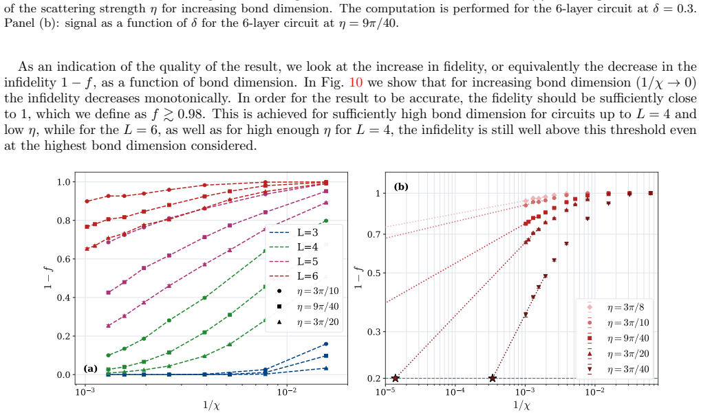
- [Classical benchmarking, Table I vs. main text] The main text states that at L=4 'TN-BP converges at a modest bond dimension chi=128 (fidelity above 0.97)', but App. B reports f≈0.974 only at chi=768 (Table I), and Fig. 10 suggests the fidelity at chi=128 is substantially lower. This discrepancy matters because Fig. 2(a) uses TN-BP at chi=128 as the ground truth for L=4. Please clarify the fidelity at chi=128 and, if it is not above 0.97, either adjust the shallow-depth claim or use a higher bond dimension for the L=4 reference.
minor comments (3)
- [Fig. 2(d), caption and axis definition] Please define precisely what 'decay factor' means when the ideal S_delta is unknown at L=6. Is it the ratio of the unmitigated signal to the globally rescaled ibm_boston reference? Without an explicit definition, the y=x line is ambiguous.
- [Eq. (1) and circuit notation] Eq. (1) writes the OLE in terms of a generic U and V_delta, while the experiment uses U = U0^dagger U_eta and V_delta placed in the middle of the echo. The main text introduces this later, but the reader would benefit from a one-line statement after Eq. (1) that the experimental circuit is a specific instance of this definition.
- [Appendices B and C] The appendix results would be easier to navigate if each classical method included a one-sentence bottom-line statement in the main text (e.g., 'MPS and TTN fail already at L=3-4'). Most of this information is present in the appendices but is slow to extract.
Circularity Check
No significant circularity: the quantum estimates are constructed from explicit, tested assumptions and validated against independent classical/exact references.
full rationale
The paper's central estimates are not forced by construction. Global rescaling is an explicit heuristic: ˜S_δ ≈ α S_δ with α estimated at δ=0, and the assumption of δ-independent attenuation is directly tested at L=3,4 against converged TN-BP and probed at L=6 via noise-manipulation stability and cross-device consistency. The cross-device consistency check treats the rescaled ibm_boston signal as a reference and cannot exclude a common δ-dependent bias; the paper itself acknowledges that small-scale tests 'do not directly validate its assumptions on the target circuits.' That is an honest limitation and a correctness risk, not a circular reduction: no equation or fitted parameter equals the claimed prediction by definition. The PEC estimates are learned from independent calibration/cycle-benchmarking data and then validated on Cliffordizations, exact δ=0 signals, and converged TN-BP at L=2,4, which are out-of-sample checks relative to the fitted noise parameters. Self-citations to prior work on sparse Pauli–Lindblad models and global rescaling are supportive but not load-bearing, since the present paper contains its own validations. The manuscript explicitly identifies and avoids the circular standard of judging a quantum computation trustworthy only when it agrees with a classical calculation. No step in the claimed derivation chain reduces to its own input.
Assumptions & free parameters
free parameters (5)
- Transverse-field angles (h, b1, b2) =
h=pi/8, b1=3pi/16, b2=0.125
- Circuit geometry (VS, VP, VO) =
|VS|=11, |VP|=35, |VO|=12
- Sparse Pauli-Lindblad noise coefficients =
per-gate Pauli error rates (Fig. 3a)
- Classical method truncations (chi, M, rc) =
chi<=980; M<=5e8; rc in {5e-2, 1e-2}
- Global rescaling factor alpha ~ S~_0 =
measured, not fitted (S~_0 at delta=0)
assumptions (8)
- standard math The OLE estimator (Eq. A6) converges to the operator trace: averaging eigenstate parities implements 2^{-n}O in the M->infinity limit.
- domain assumption Noise attenuation of the OLE signal is approximately independent of probe strength delta (global rescaling assumption: S~_delta ~ alpha*S_delta).
- domain assumption Device noise is Markovian, stochastic-Pauli, and sparse-local, represented by a sparse Pauli-Lindblad model.
- domain assumption The TN-BP fidelity estimator (Eq. B1) is a reliable convergence proxy for choosing trustworthy classical ground truth.
- domain assumption Off-diagonal OTOC contributions are negligible for the PP-MC diagonal approximation.
- standard math S_delta ~ 1 - delta^2*C/2 with higher-order moments resummed (OLE-OTOC expansion).
- domain assumption The noise channel is stable over the ~45-minute recharacterization interval.
- domain assumption Noise manipulation (gate duration, device, synthetic Pauli insertion) modifies only the noise, leaving the ideal signal unchanged.
invented entities (1)
-
Operator Loschmidt echo (OLE) as a hardware-implemented probe
independent evidence
Cite this review
Pith. "Pith review of Observable Estimation in the Absence of Classical Verification." pith.science (2026). https://pith.science/paper/IFZPLMHU
@misc{pith2026260725998,
  author       = {Pith},
  title        = {Pith review of: Observable Estimation in the Absence of Classical Verification},
  year         = {2026},
  howpublished = {\url{https://pith.science/paper/IFZPLMHU}},
  note         = {Machine review of arXiv:2607.25998}
}
read the original abstract
The predictive success of quantum mechanics underpins many areas of modern science, even as the exact simulation of large, interacting quantum systems remains beyond the reach of classical computation. This success has been enabled by the remarkable advancement of scalable numerical approximation methods, which often demonstrate practical accuracy despite the absence of formal guarantees. As quantum simulation pushes into regimes where these approximations struggle, a fundamental challenge arises: How can quantum outcomes be trusted when reliable classical benchmarks are unavailable? Here, we establish a framework for the independent validation of quantum estimates in this setting and present evidence that they provide the most credible result among several considered methods, in the absence of an immediately accessible ground-truth solution. We apply our framework to the semi-scrambling dynamics of a physical model that strains several leading classical simulation methods yet remains experimentally accessible, in part through our introduction of the \textit{operator Loschmidt echo}. We systematically design a series of experiments using quantum heuristics that, taken together, test the underlying assumptions and provide strong confidence in the observable estimates obtained from the quantum computer. We then show how this framework can be extended to place accuracy bounds on quantum estimates via careful characterization and manipulation of the device noise, transforming the problem of validating the observable estimation to validating the noise model. These results establish a route towards trusted quantum computation for scientific discovery, independent of classical verification.
Figures


Figures from the paper (34 more)








Reference graph
Works this paper leans on
-
[1]
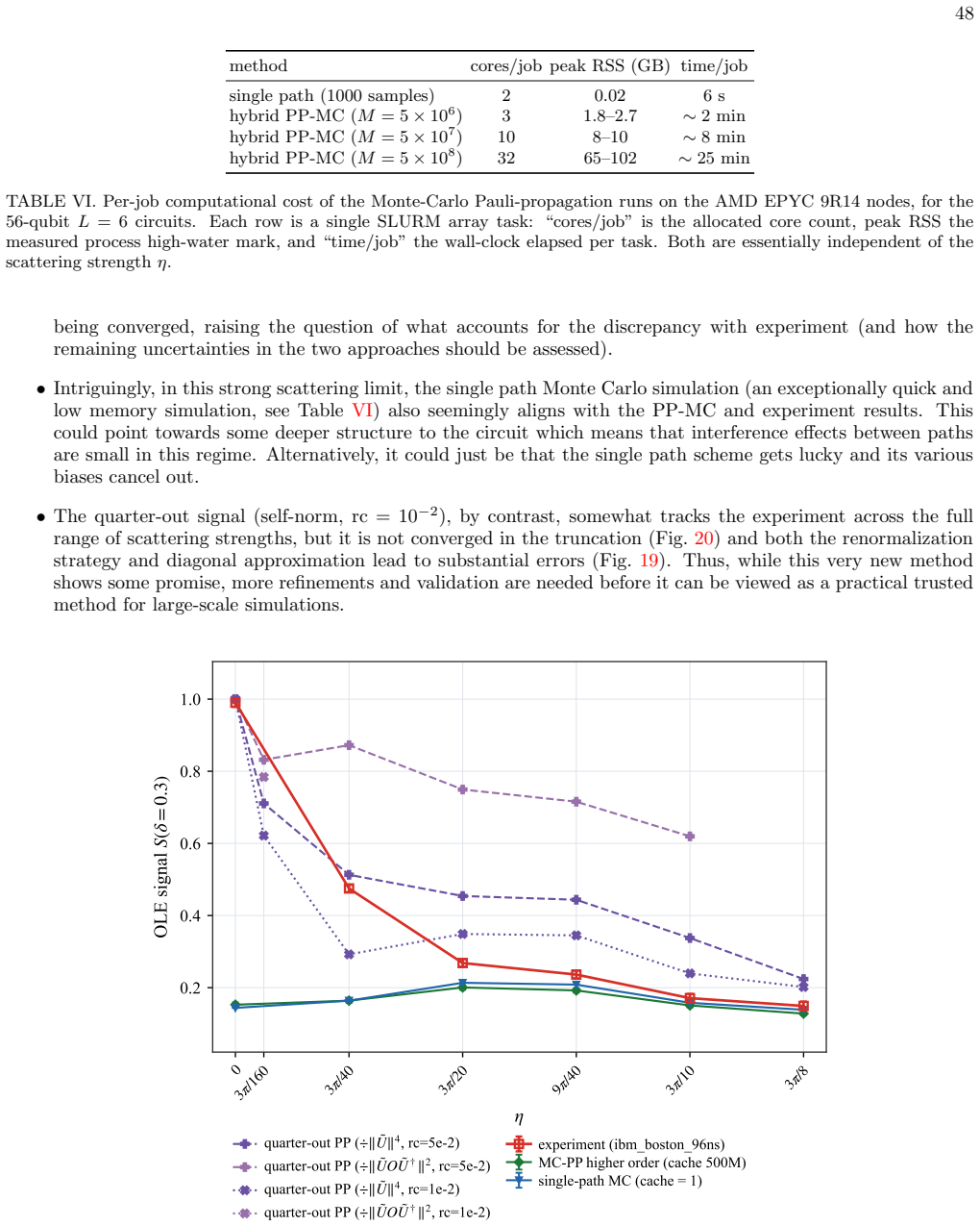
thepair-diagonalapproximation ofb 2 P [Eq. (C67)], which retains only them=a,n=bcontributions and lets each pair (a, b) contribute independently, reducing the cost from quartic to quadratic and, crucially, letting 45 1 0.12 0.14 0.16 0.18 0.20OLE signal S( = 0.3) (a) 5M 50M 250M500M cache size M 10 20 30 truncation order 2kmax 1.5 1.0 0.5 0.0 0.5 1.0 1.5 ...
-
[2]
cores/job
theapproximate self-normalizationN approx = P a |ca|2 2 =∥ ˜U∥ 4, obtained by applying the same pair- diagonal truncation to the normN( ˜U †O ˜U) = P P b2 P [Eq. (C64)]. Since the physical (normalized) estimator divides the raw pair sum by this normalization, ˆC approx 2,diag of App. C 3, and likewise every higher momentC 2m that entersS δ, the choice ofN...
-
[3]
The labelquarter-outrefers to how the operator propagation is initialized at the seam between the two halvesU 0 andU † η of the evolution
Unitary ‘quarter-out’ propagation We now consider an alternative propagation strategy based on expanding the unitaryU=U † 0 Uη itself into Pauli strings rather than sequentially propagating Pauli operators. The labelquarter-outrefers to how the operator propagation is initialized at the seam between the two halvesU 0 andU † η of the evolution. At a high l...
-
[4]
In addition to previously discussed methods, we have systematically explored other variants that led to less promising results
Summary of Pauli propagation variants explored Table V collects the Pauli-propagation variants we examined, organized along two largely independent axes: how the operator expansion is approximated, and which operator is evolved through the circuit. In addition to previously discussed methods, we have systematically explored other variants that led to less...
-
[5]
C 2) and the quarter-out unitary expansion (App
Additional numerical studies of Pauli propagation methods We now report the numerical performance of the two adopted Pauli-propagation variants, hybrid PP-MC (App. C 2) and the quarter-out unitary expansion (App. C 3), on the target semi-scrambling OLE circuits, and compare them against theibm bostonhardware data. Unless stated otherwise, all results are ...
-
[6]
Both devices are Heron (R3) architectures comprising 156 fixed- frequency transmon qubits arranged in a heavy-hexagonal connectivity
Superconducting Quantum Hardware Experiments were performed onibm bostonandibm pittsburgh, which are superconducting quantum processors available through the IBM Quantum Platform. Both devices are Heron (R3) architectures comprising 156 fixed- frequency transmon qubits arranged in a heavy-hexagonal connectivity. Qubit coherence times are shown in Fig. 24....
-
[7]
Therefore, the CZ gates were calibrated with identical pulse duration and parallelized using the three sets of matching batches of gates [4]
Two-Qubit Gate Calibrations The OLE circuit consists of repetitions of three unique layers of CZ gates. Therefore, the CZ gates were calibrated with identical pulse duration and parallelized using the three sets of matching batches of gates [4]. Calibration included optimization of theZZ,IZ, andZIrotation angles effectuated by the gate pulse, as determine...
-
[8]
Figure 25 demonstrates transient gate errors as a function of delay times between CZ gates
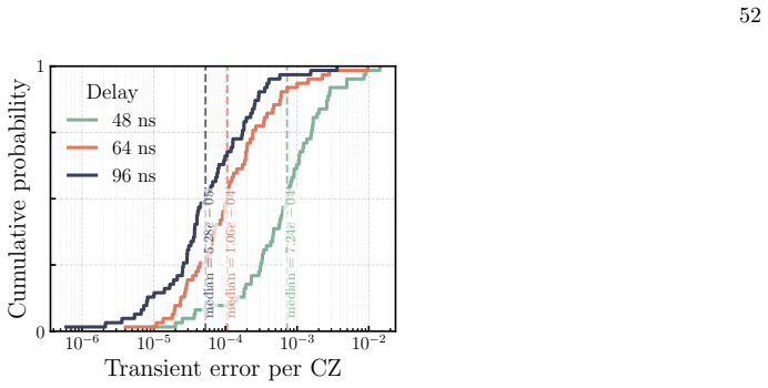
Gate T ransient Errors Pulse transients due to signal distortions in flux control lines may impart coherent errors to CZ gates and are a source of non-Markovianity that is particularly a challenge for noise learning and PEC. Figure 25 demonstrates transient gate errors as a function of delay times between CZ gates. This implies that the noise model learne...
Show all 14 references
-
[9]
Noise stabilization For PEC experiments, drift in the landscape of two-level system defects (TLS) between noise model learning and target-circuit execution could cause changes in the noise channel and therefore invalidation of the learned model. To stabilize the noise channel,...
-
[10]
node-based
Post-selection of non-Markovian leakage errors Error mitigation protocols often rely on having a representative model of the device noise that is informed by an experimental noise learning step. An efficient Pauli noise-learning protocol based on the sparse Pauli-Lindblad nois...
-
[11]
Recall that the OLE circuits are decomposed into CZ, R Z(2h), and RX (2b) whereh=π/8 andb∈ {b 1, b2, b1 −η}
Cliffordizations In our experiments, we useCliffordizationsof our target circuit to calibrate and validate the noise models [112]. Recall that the OLE circuits are decomposed into CZ, R Z(2h), and RX (2b) whereh=π/8 andb∈ {b 1, b2, b1 −η}. A Cliffordization of the OLE circuit ...
-
[12]
Model Fit Observables
Maintaining an Accurate Noise Model In the idealized limit where the learned noise model coincides with the true device noise, probabilistic error cancellation (PEC) yields unbiased expectation values with rigorous error bounds [14]. In practice, however, device noise may have...
-
[13]
Current rates
Shaded lightcones Standard PEC [14, 15] inverts every error channel in the circuit, including channels that commute with the observable and therefore leave its expectation value unchanged. Mitigating these channels wastes sampling overhead. The Shaded Lightcone (SLC) [31, 119]...
2000
-
[14]
39q” “44q 0
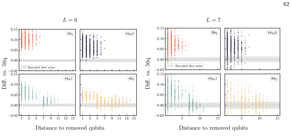
Error propagation As mentioned earlier, if noise learning were exact, the error of a PEC-mitigated estimate would be purely statistical. In practice the learned ratesλ P carry both statistical uncertainty, from the finite number of cycle-benchmarking shots, and systematic erro...
Reviewed August 1, 2026 · model on record in the stance chip above.
Discussion (0). Sign in to comment.