REVIEW 1 major objections 3 minor 14 references
Online Conformal Prediction Beyond Feedback
T0 review · 1 major / 3 minor · reviewed 2026-08-10 · deepseek-v4-flash
Pith's one-line read This paper shows that online conformal prediction can keep a user-specified coverage guarantee even when no deployed prediction set is ever evaluated, by querying the true label on only an expected $T^{-1/3}$ fraction of rounds.
desk verdict Strong expected-coverage result for a genuinely new query-only OCP setting; the high-probability companion proof has a real concentration gap that needs fixing. read the letter →
The pith
A machine-rendered reading of the paper's core claim, the machinery that carries it, and where it could break.
The reading
What carries the argument
The load-bearing objects are the auxiliary reward function $R(m,t)$ and the inverse-probability estimator $\hat{X}_{m,t}$. For threshold $m$ on round $t$, $R(m,t)=0$ if the true label is outside the set $\Gamma_C(x_t,m)$, and otherwise $1-m(1-\beta)$; the query action always gets reward zero. When a query is made, $R(m,t)$ is revealed for all $m$ simultaneously, and the update $\hat{Z}_{m,t+1}=\hat{Z}_{m,t}+\hat{X}_{m,t}$ with $\hat{X}_{m,t}=1-\frac{1-R(m,t)}{\epsilon}$ on query rounds keeps cumulative reward estimates unbiased (Lemma 1). The exponentially weighted mix over thresholds then drives regret to the optimal $\Theta(T^{2/3})$ rate for this partial monitoring game.
What would settle it
Run OCPQ on a stream produced by an adaptive adversary that makes each label depend on whether the learner queried or predicted on previous rounds, for example by selecting the lowest-probability class under $C$ precisely on rounds that follow a query; if the expected coverage falls below $\beta - O(T^{-1/3})$ for large $T$, the oblivious-stream assumption is the reason and the central guarantee does not hold.
Extended reading notes
Core claim
The paper's central claim is Corollary 1: on any oblivious stream $z^T$, for any classifier $C$, any finite threshold set $\mathcal{M}\ni\{0,1\}$, and any target $\beta\in[0,1]$, the OCPQ algorithm with $\epsilon=T^{-1/3}$ and $\eta=T^{-2/3}\sqrt{\ln|\mathcal{M}|}$ satisfies $\mathbb{E}[p_{\mathrm{cover}}]\ge \beta - (2\sqrt{\ln|\mathcal{M}|}+1)/T^{1/3}$, while querying an expected $T^{-1/3}$ fraction of rounds. The algorithmic step is to treat prediction thresholds as experts and the query action as an observation-only arm; a query reveals the auxiliary reward $R(m,t)$ of every threshold at once, and inverse-probability weighting keeps the cumulative estimates unbiased. The resulting $O(T^{2/3})$ expected regret is converted into coverage by noting that the always-safe threshold $m=1$ collects $\beta$ per round, so low regret forces coverage close to $\beta$.
Load-bearing premise
The data stream is fixed in advance: the inputs and labels cannot respond to the learner's past queries or predictions, and every query must return the exact true label.
Editorial extensions
If this is right
- Every black-box classifier gains a finite-horizon coverage guarantee even though no deployed prediction set is ever evaluated.
- Users can set the target coverage through $\beta$ and, since the deficit term is explicit, can inflate $\beta$ to compensate for finite $T$.
- The $O(T^{2/3})$ expected regret is asymptotically optimal for the induced partial monitoring game when $\beta<1$, so this protocol cannot be solved at a faster rate by any algorithm.
- The coverage lower bound also holds with high probability, by Theorem 3 and Corollary 2, not only in expectation.
- Only an expected $T^{-1/3}$ fraction of rounds requires a label, making the method suited to settings where labels are expensive or arrive only through deferral.
Reading between the lines
- A data-dependent query rate is a natural follow-up: the proof only needs $\epsilon$ tuned to $T$, so a scheme that lowers $\epsilon$ as the best-threshold estimate stabilises could reduce label cost while preserving the $O(T^{-1/3})$ deficit, although the authors do not analyse this.
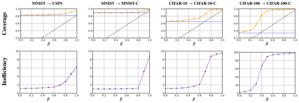
- Because the guarantee is relative to the best threshold in a fixed finite grid $\mathcal{M}$, an adaptive grid that refines around the current favourite should improve efficiency without extra queries; the sensitivity experiments suggest diminishing returns beyond about 64 thresholds.
- The sigmoidal coverage-versus-$\beta$ curves reported in the experiments imply that calibration of $\beta$ is delicate; a practical extension would be a short burn-in phase to estimate the inflection point before committing to $\beta$.
- If the adversary is made adaptive, I would expect the unbiased estimator argument in Lemma 1 to break, so the paper's coverage bound should be read as tied to the oblivious-stream model rather than as a fully adversarial guarantee.
Signed reviews
Editorial analysis
A structured set of objections, weighed in public.
Referee Report
Summary. The paper introduces OCPQ, an online conformal prediction method for a 'beyond feedback' protocol: on each round the learner either outputs a prediction set or queries the true label, but never both, so no deployed prediction is ever evaluated. The problem is reduced to a finite partial-monitoring game whose actions are prediction thresholds plus a query action, and OCPQ adapts the label-efficient forecaster of Cesa-Bianchi, Lugosi, and Stoltz (2004) to this setting. The main theoretical claims are an expected regret bound of O(T^{2/3}) (Theorem 1), a reduction from regret to coverage (Theorem 2), an expected coverage guarantee p_cover >= beta - O(T^{-1/3}) at an expected query fraction T^{-1/3} (Corollary 1), and high-probability versions of the regret and coverage bounds (Theorem 3 and Corollary 2). Experiments on distribution-shift benchmarks and on LLM safety-monitoring prompts with adversarial rewrites illustrate the coverage-efficiency trade-off and compare with full-feedback ACI.
Significance. The expected-coverage guarantee in Corollary 1 is a meaningful and clearly stated contribution: it provides finite-horizon coverage control for online conformal prediction when deployed prediction sets produce no feedback, at the price of an O(T^{-1/3}) coverage deficit and an O(T^{-1/3}) query rate. I checked the key algebra of Theorems 1 and 2 and found the expected-regret and regret-to-coverage arguments sound: Lemma 1 establishes the unbiasedness of the estimator, and the derivation of Corollary 1 from the two theorems is valid. The paper is also honest about its modeling assumptions, explicitly acknowledging the oblivious-adversary restriction and the fact that queries count as miscoverage events. The experimental section is substantial and includes a realistic LLM safety-monitoring application. However, the advertised high-probability result (Theorem 3 and Corollary 2) is not proven as written, because the concentration argument applies Hoeffding's inequality to history-dependent random variables and combines dependent probability events by multiplication.
major comments (1)
- [Appendix: Proofs, Theorem 3] The proof of Theorem 3 is invalid as written. Hoeffding's inequality is applied to r1 = R_{T,pi}/T and to r2 = (1/Q) * sum_{t: a_t=query} sum_{m in M} P_{m,t} R(m,t), but these are not averages of independent bounded random variables: the action A_t at time t is sampled from a distribution P_{m,t} that depends on all previous observations, and the terms inside r2 share the same history and are divided by the random quantity Q. Consequently the displayed inequalities such as P(E[R_{T,pi}]/T - lambda >= r1) and P(r2 - E[r2] >= lambda) <= exp(-2 Q lambda^2) do not follow. In addition, the proof uses the identity E[r1] = (1-epsilon) E[r2] as exact, but this does not follow by linearity of expectation because the denominator Q in r2 is random and correlated with the numerator. Finally, the final probability in Eq. (8) is obtained by multiplying two success probabilities for events that are not independent; a union bound would give a sum of failure probabilities, not a product. As a result, Theorem 3 and Corollary 2 are not established. This is load-bearing because these high-probability guarantees are explicitly listed among the paper's contributions and are used to argue that OCPQ has no pathologically high variance.
minor comments (3)
- [Appendix: Corollary 2] The sign of the 2*T^{-1/4} term in the coverage bound in the appendix is inconsistent with the main-text version and with the derivation from Theorem 3: it should be minus, not plus.
- [Appendix: Proofs, Theorem 3] In the expansion of tilde{R}_{T,pi} - R_{T,pi}, the line containing 'T*(r2 - r2)' should read 'T*(r2 - r1)'; as printed it is a typo that obscures the argument.
- [Appendix: Proofs, Theorem 1] The statement that the distribution of hat{X}_{A_t,t} 'only depends on epsilon, x_t, y_t, and C' is imprecise because hat{X} also depends on the action A_t. The needed independence between P_{m,t} and hat{X}_{m,t} holds because the query indicator at time t is independent of the history that determines P_{m,t}; the proof should say this explicitly.
Circularity Check
No significant circularity: the coverage guarantee is derived from the regret bound and the reward design, not assumed or fitted.
full rationale
The central claim, Corollary 1, is obtained by chaining Theorem 1, an expected-regret bound for the label-efficient forecaster adapted to the query/prediction protocol, with Theorem 2, which converts regret under the auxiliary reward of Definition 1 into a coverage lower bound. This conversion is not circular: threshold m=1 always covers, so R(1,t)=β; any action's reward is at most 1 on a covered prediction and 0 on a query or miscoverage; hence total reward is at most pcover·T, giving βT − reward ≤ regret, and therefore pcover ≥ β − regret/T. The parameter β is deliberately injected into the reward to make this reduction valid, but the algorithm is not fitted to coverage data and the bound is not assumed as an input. Lemma 1's unbiasedness is proved from the query probability ε, not postulated. No load-bearing self-citation appears: the learning rule is credited to Cesa-Bianchi, Lugosi, and Stoltz (2004), and the authors' own prior works are cited only for motivation and related protocols. The lower-bound optimality claim in Proposition 2 imports Lattimore and Szepesvari (2018), an external source, and the proof directly checks global observability and non-local observability. The suspected flaw in the high-probability proof of Theorem 3, namely the application of Hoeffding's inequality to history-dependent averages r1 and r2, is a correctness concern rather than a circularity; it does not affect the expected-coverage derivation. Accordingly, no circular step is identified.
Assumptions & free parameters
free parameters (4)
- epsilon (query rate) =
T^{-1/3}
- eta (learning rate) =
T^{-2/3} sqrt(ln|M|)
- beta (coverage baseline) =
user-specified in [0,1]
- M (threshold set) =
finite subset of [0,1] containing 0 and 1
assumptions (5)
- domain assumption Oblivious adversary: the data stream z^T = (x_t,y_t) is fixed in advance and independent of the algorithm's actions.
- domain assumption The query action always reveals the true label y_t exactly.
- domain assumption Y is finite and the classifier C outputs a probability distribution over Y.
- ad hoc to paper 1 is in M and the auxiliary reward is R(m,t)=1-m(1-beta) for coverage events and 0 otherwise.
- standard math Standard concentration inequalities (Hoeffding) and algebraic inequalities (e^x <= 1+x+x^2 for x <= 1) used in the proofs.
Cite this review
Pith. "Pith review of Online Conformal Prediction Beyond Feedback." pith.science (2026). https://pith.science/paper/IGSIZ35Z
@misc{pith2026260807139,
  author       = {Pith},
  title        = {Pith review of: Online Conformal Prediction Beyond Feedback},
  year         = {2026},
  howpublished = {\url{https://pith.science/paper/IGSIZ35Z}},
  note         = {Machine review of arXiv:2608.07139}
}
abstract
Uncertainty quantification is essential when deploying machine learning models in safety-critical applications. Online conformal prediction (OCP) provides theoretically principled uncertainty quantification for arbitrary black-box classifiers and non-i.i.d. data streams by constructing prediction sets that are guaranteed to contain the true label at a user-specified frequency. OCP usually updates prediction sets using feedback from previously deployed predictions. We instead study an OCP setting beyond feedback: on each round, the learner can either output a prediction set or query the correct label, but not both. Thus, no deployed prediction is ever evaluated directly. We reduce this problem to a partial monitoring game in which prediction actions return no observation and a separate query action reveals the label. The reward function is constructed in a way that encourages the learner to output small prediction sets while ensuring that the correct label is covered with a sufficiently high probability. To solve this game, we develop OCP with queries (OCPQ) by adapting the label efficient forecaster of Cesa-Bianchi, Lugosi, and Stoltz (2004) to our setting. For any black box classifier and any (non-i.i.d.) oblivious data stream of length $T$, OCPQ has $O(T^{2/3})$ expected regret and expected coverage at least $\beta-O(T^{-1/3})$ for a user-defined $\beta$, while querying only an expected $T^{-1/3}$ fraction of rounds. This provides coverage comparable to bandit-based OCP methods while requiring no feedback from deployed prediction sets. Experiments on real-world datasets further demonstrate the effectiveness of our approach.
Figures


Figures from the paper (7 more)



Reference graph
Works this paper leans on
-
[1]
For convenience, let C(x, y) =C(x)y
We assume that we have a classifierC:X→∆(Y), so thatC(x)is a distribution overY. For convenience, let C(x, y) =C(x)y
-
[2]
Safe Planning in Dynamic Environments using Con- formal Prediction. arXiv:2210.10254. McKenzie,A.;Pawar,U.;Blandfort,P.;Bankes,W.;Krueger, D.; Lubana, E. S.; and Krasheninnikov, D. 2026. De- tecting High-Stakes Interactions with Activation Probes. arXiv:2506.10805. Mu, N.; and Gilmer, J. 2019. MNIST-C: A Robustness Benchmark for Computer Vision. arXiv:190...
arXiv 2026
-
[3]
Oneachround,weobserveanx t.Ifwemakeaquery,we alsoobservey t.Otherwise,wepickapredictionthreshold mt ∈M, and let St ={y∈Y:C(y, x t)≥max y⋆ C(y ⋆, xt)−m t}. We must also specify the action space, observation space, and state space. We could let the statesSrepresentxandy directly, but this becomes very unwieldy, so we will instead let the state at timetcorre...
work page 2019
-
[4]
Let ˜RT,π be the “pseudo-expected regret” of the learner, i.e., ˜RT,π = TX t=1 KX i=1 Pi,t · ˆXi,t, whereP m,t = expη ˆZm,t/ P i∈M expη ˆZi,t
-
[5]
We discretise[0,1]into a finite set ofprediction thresh- oldsM⊂[0,1]
-
[7]
0 ifGhas no pairs of neighbouring actions, 2.Θ(T 1/2)ifGislocallyobservableandhasneighbouring actions, 3.Θ(T 2/3)ifGis globally observable but not locally ob- servable, and 4.Θ(T)otherwise, see Theorem 1 in Lattimore and Szepesvari (2018). This proof will use terminology from Lattimore and Szepesvari (2018),butforthesakeofbrevitywewillnotdefinethister- mi...
work page 2018
-
[8]
if some thresholdmgets a lot of reward, thenˆZm,T+1, and hencew m,T+1, and henceW T+1 will be large in expectation, and
-
[9]
ln|M| η +η TX t=1 X m∈M Pm,t · ˆX 2 m,t # = ln|M| η +η TX t=1 E
if the learner does not get a lot of reward in expectation, thenW T+1 will be small in expectation. Together, this can be used to bound the expected reward of thelearningalgorithmintermsofthetotalrewardofthebest individual prediction threshold. In this proof, it will be convenient to distinguish between theactionprobabilitiesthataresuggestedbytheexponenti...
Show all 14 references
-
[10]
LetR T,m be the total reward of prediction thresholdm, i.e., PT t=1 R(m, t)
-
[11]
LetR T,π bethe(random)totalrewardofthelearner,i.e.,PT t=1 R(At, t)
-
[12]
Let ˆRT,m be the total estimated reward of armi, i.e., ˆZm,T+1
-
[14]
pseudo-expected reward
Let REGm be the random regret that learner suffers with respect to prediction thresholdm(so, i.e., REG m = RT,m −R T π). We then have that REGm =R T,m −R T,π =R T,m −R T,π + ( ˆRT,m − ˆRT,m ) + ( ˜RT,π − ˜RT,π ) = ( ˆRT,m − ˜RT,π )+ (RT,m − ˆRT,m ) + ( ˜RT,π −R T,π ) ≤ ln|M| η...
2004
-
[2023]
Ge,H.;Bastani,H.;andBastani,O.2025
Calibrating AI Models for Wireless Communications via Conformal Prediction.IEEE Transactions on Machine Learning in Communications and Networking, 1: 296–312. Ge,H.;Bastani,H.;andBastani,O.2025. StochasticOnline ConformalPredictionwithSemi-BanditFeedback. InSingh, A.; Fazel, M...
2025 arXiv
-
[2026]
arXiv:2507.11878
LLMs Encode Harmfulness and Refusal Separately. arXiv:2507.11878. Zhao, M.; Simmons, R.; Admoni, H.; Ramdas, A.; and Ba- jcsy, A. 2025. Conformalized Interactive Imitation Learn- ing: Handling Expert Shift and Intermittent Feedback. arXiv:2410.08852. Zhu,M.;Zecchin,M.;Park,S.;...
2020 arXiv
Reviewed August 10, 2026 · model on record in the stance chip above.
Discussion (0). Continue with ORCID to comment.