REVIEW 4 minor 32 references
Magnetic helicity in multiply connected domains
T0 review · 0 major / 4 minor · reviewed 2026-08-14 · deepseek-v4-flash
Pith's one-line read Magnetic helicity has a gauge-invariant definition for any bounded multiply connected domain in three-dimensional space.
desk verdict A clean, checkable unification of Bevir-Gray and Biot-Savart helicity for multiply connected domains; the main formula is new and the mathematics holds up, with one soft spot in the mutual-helicity section. read the letter →
The pith
A machine-rendered reading of the paper's core claim, the machinery that carries it, and where it could break.
The reading
What carries the argument
The central mechanism is the Helmholtz decomposition for multiply connected domains, which expresses any vector-potential difference as $\operatorname{grad}\chi + \rho$, where $\rho$ lies in the finite-dimensional space of Neumann harmonic fields satisfying $\operatorname{curl}\rho=0$, $\operatorname{div}\rho=0$, and $\rho\cdot n=0$. Combined with a boundary decomposition of tangential traces in terms of the harmonic-field traces $\rho_j\times n$ and $\rho'_j\times n$, and the biorthogonality identity $\int_{\partial\Omega} \rho_j\times n\cdot \rho'_i = \delta_{ij}$, the gauge variation of $\int_\Omega A\cdot B$ becomes exactly the flux-weighted circulation sum in equation (2.17). The Biot-Savart operator then removes that sum because its line integrals around the cycles $\gamma_j$ vanish on the exterior side of the domain.
What would settle it
Compute, for a solid torus or toroidal shell, the pairing integrals $\int_{\partial\Omega}(\rho_j\times n)\cdot\rho'_i$ directly from the harmonic-field basis used in the paper; if any differs from $\delta_{ij}$, equation (2.20) is not gauge invariant. Alternatively, for a field carrying only poloidal flux, evaluate $\int_\Omega A\cdot B$ under two different vector potentials and check whether subtracting the flux-weighted circulations gives the same number and equals $\int_\Omega BS(B)\cdot B$.
Extended reading notes
Core claim
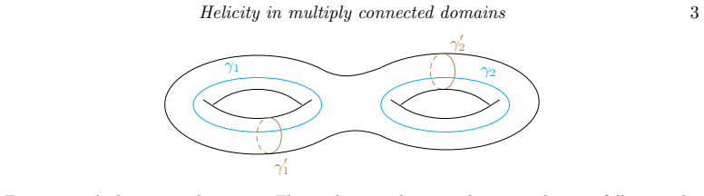
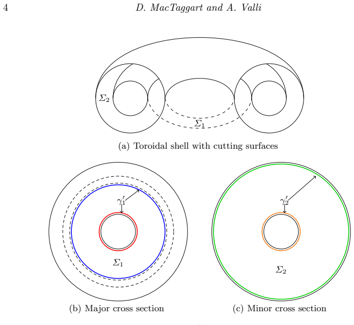
The paper claims that the quantity $\Upsilon(B) = \int_\Omega A\cdot B - \sum_{j=1}^g \left(\oint_{\gamma_j} A\cdot t_j\right)\left(\int_{\Sigma_j} B\cdot n_j\right)$ is the gauge-invariant magnetic helicity for every bounded connected Lipschitz domain in $\mathbb{R}^3$, where $\gamma_j$ are homology cycles of the domain, $\Sigma_j$ are cutting surfaces bounded by companion cycles, and $B\cdot n=0$ on $\partial\Omega$. The formula reduces to the classical Bevir-Gray expression when $g=1$, to the ordinary volume integral when all cutting-surface fluxes vanish or the domain is simply connected, and to the Biot-Savart helicity $\int_\Omega BS(B)\cdot B$ when the vector potential is chosen as $BS(B)$. The paper also shows that the general mutual helicity formula follows from the same expression, reproducing known flux-and-linking-number formulas for linked domains.
Load-bearing premise
The derivation depends on the boundary traces of two families of harmonic fields pairing exactly as $\delta_{ij}$; if that normalization fails for some domain, the cancellation that produces the generalized Bevir-Gray formula is no longer exact and $\Upsilon(B)$ would acquire unwanted extra terms.
Editorial extensions
If this is right
- In any multiply connected domain, the ordinary integral $\int_\Omega A\cdot B$ is not the helicity; the correct invariant subtracts, for each homology cycle, the circulation of the vector potential around that cycle times the magnetic flux through the corresponding cutting surface.
- With the Biot-Savart potential, the correction term vanishes automatically, so helicity becomes $\int_\Omega BS(B)\cdot B$ without imposing any zero-flux condition.
- The general formula reduces to the Bevir-Gray expression for a torus and to the standard volume integral in simply connected domains or when all relevant fluxes vanish.
- Mutual helicity between two linked domains follows directly from the same formula and is expressible as flux products weighted by linking numbers, matching the known general mutual helicity formula.
- Periodic simulation domains that are topologically tori or toroidal shells inherit the correction terms, while triply periodic cubes, which cannot be embedded in $\mathbb{R}^3$, lie outside the scope of the formula.
Reading between the lines
- I infer that the formula gives a practical numerical recipe: any gauge can be used in a computation, provided the flux-weighted circulation terms are subtracted, avoiding the expense of constructing the Biot-Savart potential directly.
- If the biorthogonality normalization is only approximate in a discrete setting, the paper's identities suggest a diagnostic: monitor the pairing integrals $\int_{\partial\Omega} \rho_j\times n\cdot \rho'_i$ to control gauge-invariance error in computed helicities.
- The same correction structure likely applies to other Hodge-type invariants, such as fluid helicity or cross-helicity, in multiply connected fluid domains, where analogous flux terms would appear.
Signed reviews
Editorial analysis
A structured set of objections, weighed in public.
Referee Report
Summary. The paper proposes a gauge-invariant definition of magnetic helicity for bounded connected domains in R^3 with Lipschitz boundary, allowing for arbitrary first Betti number. Using the Helmholtz decomposition and Neumann harmonic fields, the authors derive the formula Υ(B) = ∫_Ω A·B − Σ_{j=1}^g (∮_{γ_j} A·t_j)(∫_{Σ_j} B·n_j) (Eq. 2.20), generalizing the Bevir-Gray formula. They further show that when the vector potential is the Biot-Savart operator, the correction term vanishes for n-holed tori and toroidal shells, so that Υ reduces to ∫_Ω BS(B)·B. The paper also discusses field line helicity on toroidal boundaries and derives a mutual helicity formula, proving the two-linked-tori case and asserting equivalence with Cantarella's general formula.
Significance. If the result holds, it unifies two previously separate approaches to helicity in multiply connected domains: the plasma-physics Bevir-Gray construction and the geometric Biot-Savart construction. The paper is careful and explicit about the topology, with a detailed treatment of cutting surfaces for n-holed tori and toroidal shells, and it clearly specifies orientation conventions. The stepwise derivations in Sections 2.4 and 2.5 are mathematically sound, and the resulting formula is directly applicable to MHD problems in toroidal and periodic domains. The paper also provides physical interpretations via boundary field line helicity, which strengthens its interest for the plasma physics community.
minor comments (4)
- [Section 2.4, Eqs. (2.10)–(2.12)] The biorthogonality relation ∫_∂Ω ρ_j×n·ρ'_i = δ_ij is imported from Alonso Rodríguez et al. (2018) without proof. Since the coefficient evaluation leading to Eq. (2.12), and hence the main formula (2.20), depends on the normalization and sign of this relation, please state the precise theorem with the orientation conventions used, or provide a short proof in an appendix, so that the signs in (2.12) can be independently verified.
- [Section 2.6, Eq. (2.43)] The claim that Eq. (2.43) is equivalent to Cantarella's general mutual helicity formula is only sketched ("a careful analysis of the values of the linking numbers... would show") and is demonstrated only for the special case of two linked solid tori. Since this is an advertised result of the paper, please either provide the general argument or explicitly state the scope of the proven result.
- [Introduction and Section 2.1] There are several typographical errors: "and and" in the Introduction, "geometical" in Section 2.1, and "contruction" in Section 2.2. These should be corrected.
- [Section 2.5.2] The sentence "Applying this result to the Biot-Savart vector field BS(B), for which (from (2.25)), ∮_{γ1} BS(B)·t1 = 0" reads awkwardly and the equation reference formatting is unclear; consider rewriting as "for which ∮_{γ1} BS(B)·t1 = 0 by (2.25)."
Circularity Check
No circularity: the generalized helicity formula is derived from the Helmholtz decomposition and standard biorthogonality identities, not assumed as an input.
full rationale
The central formula (2.20) is not introduced as a definition that already contains the answer; it is obtained by an explicit computation of H1 - H2. The gauge-invariance proof is a direct calculation: equations (2.9)-(2.17) show that the difference of helicities with two vector potentials equals a sum of products of circulation differences and fluxes, so the combination in (2.20) is invariant by construction, not by assumption. The only imported ingredients are the Helmholtz decomposition (Theorem 1), the construction and biorthogonality of Neumann harmonic fields from Alonso Rodríguez et al. (2018), and the extension property of the Biot-Savart operator from Cantarella et al. (2001). Although A. Valli is a co-author of the cited Alonso Rodríguez et al. paper and of Valli (2019), these citations are used for standard Hodge-theoretic facts and for the Biot-Savart extension, both of which are parameter-free mathematical statements that do not presuppose the target formula. The reduction to Biot-Savart helicity is proved via Stokes' theorem: since each cycle gamma_j bounds a surface Sigma'_j in the exterior domain Omega' where curl BS(B) = 0, the line integrals (2.25) vanish, making (2.20) coincide with (2.26). This is a genuine theorem rather than a renamed input. The mutual-helicity formula in Section 2.6 is derived from (2.20) and is explicitly compared with Cantarella (2000), not used as an input. No fitted parameter, self-referential definition, or author-imported uniqueness theorem carries the argument. Therefore the paper exhibits no significant circularity.
Assumptions & free parameters
assumptions (5)
- standard math Helmholtz decomposition: every u in (L^2(Ω))^3 can be written as curl P + grad φ + ρ with ρ a Neumann harmonic field (Theorem 1, Section 2.2).
- standard math The Neumann harmonic field bases {ρ_j} and {ρ'_j} for Ω and Ω' satisfy the boundary biorthogonality identities listed in equations (2.10)-(2.12), including ∫_∂Ω ρ_j × n · ρ'_i = δ_ij.
- standard math The Biot-Savart operator BS maps V into V and satisfies curl BS(B) = B̃, the zero-extension of B to R^3.
- domain assumption The domain Ω is a bounded connected open set with Lipschitz boundary, and the magnetic field B lies in V = {B ∈ (L^2(Ω))^3 : div B = 0, B·n = 0 on ∂Ω}.
- domain assumption Each non-bounding cycle γ_j of Ω bounds a surface Σ'_j contained in the complementary domain Ω'.
Cite this review
Pith. "Pith review of Magnetic helicity in multiply connected domains." pith.science (2026). https://pith.science/paper/IJI33KSO
@misc{pith2026190803721,
  author       = {Pith},
  title        = {Pith review of: Magnetic helicity in multiply connected domains},
  year         = {2026},
  howpublished = {\url{https://pith.science/paper/IJI33KSO}},
  note         = {Machine review of arXiv:1908.03721}
}
abstract
Magnetic helicity is a fundamental quantity of magnetohydrodynamics that carries topological information about the magnetic field. By `topological information', we usually refer to the linkage of magnetic field lines. For domains that are not simply connected, however, helicity also depends on the topology of the domain. In this paper, we expand the standard definition of magnetic helicity in simply connected domains to multiply connected domains in $\mathbb{R}^3$ of arbitrary topology. We also discuss how using the classic Biot-Savart operator simplifies the expression for helicity and how domain topology affects the physical interpretation of helicity.
Figures
Reference graph
Works this paper leans on
-
[1]
Alonso Rodr´ıguez, A., Cama˜no, J., Rodr´ıguez, R., Valli, A. & Venegas, P. 2018 Finite element approximation of the spectrum of the curl operator in a multiply connected domain. Found. Comput. Math. 18 1493–1533
work page 2018
-
[2]
Arnold, V. I. & Khesin, B. A. 1992 Topological methods in hydrodynamics. Annu. Rev. Fluid Mech. 24 145–146
work page 1992
-
[3]
Benedetti, R., Frigerio, R. & Ghiloni, R. 2012 The topology of Helmholtz domains, Expo. Math. 30 319–375
work page 2012
-
[4]
Berger, M. A. & Field, G. B. 1984 The topological properties of magnetic helicity. J. Fluid Mech. 14 133-148
work page 1984
-
[5]
A, 1984 Rigorous new limits on magnetic helicity dissipation in the solar corona
Berger, M. A, 1984 Rigorous new limits on magnetic helicity dissipation in the solar corona. Geophys. Astrophys. Fluid Dyn. 30 79–104
work page 1984
-
[6]
Berger, M. A. 1988 An energy formula for nonlinear force-free magnetic fields. Astron. Astrophys. 201 355–361
work page 1988
-
[7]
Berger, M. A. 1997 Magnetic helicity in a periodic domain. J. Geophys. Res. 102 2637–2644
work page 1997
- [8]
Show all 32 references
-
[9]
1993 Nonlinear magnetohydrodynamics
Biskamp, D. 1993 Nonlinear magnetohydrodynamics. Cambridge University Press
1993
-
[10]
A., Friedrichs, K
Blank, A. A., Friedrichs, K. O. & Grad, H. 1957 Notes on magneto-hydrodynamics V. Theory of Maxwell’s equations without displacement current. AEC Research and Development Report NYO-6486
1957
-
[11]
& Teytel, M
Cantarella, J., DeTurck, D., Gluck, H. & Teytel, M. 2000 Isoperimetric problems for the helicity of vector fields and the Biot-Savart and curl operators. J. Math. Phys. 41 5615–5641
2000
-
[12]
2000 A general mutual helicity formula
Cantarella, J. 2000 A general mutual helicity formula. Proc. Roy. Soc. Lon. A 456 2771–2779 14 D. MacTaggart and A. Valli
2000
-
[13]
& Gluck, H
Cantarella, J., DeTurck, D. & Gluck, H. 2001 The Biot-Savart operator for application to knot theory, fluid dynamics and plasma physics. J. Math. Phys. 42 876–905
2001
-
[14]
& Gluck, H.2002 Vector calculus and the topology of domains in 3-space
Cantarella, J., DeTurck, D. & Gluck, H.2002 Vector calculus and the topology of domains in 3-space. Amer. Math. Monthly 105 409–442
2002
-
[15]
Chui, A. Y. K. & Moffatt, H. K. 1995 The energy and helicity of knotted magnetic flux tubes. Proc. R. Soc. Lond. A 451 609–629
1995
-
[16]
& Vela-Vick, D
DeTurck, D., Gluck, H., Komendarczyk, R., Melvin, P., Shonkwiler, C. & Vela-Vick, D. S. 2013 Generalized Gauss maps and integrals for three-component links: Toward higher helicities for magnetic fields and fluid flows. J. Math. Phys. 54 013515
2013
-
[17]
L., Yoshida, Z., Bhattacharjee, A
Dewar, R. L., Yoshida, Z., Bhattacharjee, A. & Hudson, S. R. 2015 Variational formulation of relaxed and multi-region relaxed magnetohydrodynamics. J. Plasma Phys. 81 515810604
2015
-
[18]
1998 Topology, matter and space 1: Topological notions in 19th-century natural philosophy
Epple, M. 1998 Topology, matter and space 1: Topological notions in 19th-century natural philosophy. Arch. Hist. Exact Sci. 52 297–392
1998
-
[19]
& Lindberg, S
Faraco, D. & Lindberg, S. 2018 Proof of Taylor’s Conjecture on Magnetic Helicity Conservation. Commun. Math. Phys. https://doi.org/10.1007/s00220-019-03422-7
2018 doi
-
[20]
2004 The geometry of physics
Frankel, T. 2004 The geometry of physics. Cambridge University Press
2004
-
[21]
Gross, P. W. & Kotiuga, P. R. 2004 Electromagnetic Theory and Computation: A Topological Approach. Cambridge University Press
2004
-
[22]
R & Tordeux, S
Hiptmair, R., Kotiuga, P. R & Tordeux, S. 2012 Self-adjoint curl operators. Ann. Mat. Pura Appl. 191 431–457
2012
-
[23]
S., Browning, P
Hussain, A. S., Browning, P. K. & Hood, A. W. 2017 A relaxation model of coronal heating in multiple interacting flux ropes. Astron. Astrophys. 600 A5
2017
-
[24]
& Ito, N
Jordan, R., Yoshida, Z. & Ito, N. 1998 Statistical mechanics of three-dimensional magnetohydrodynamics in a multiply connected domain. Physica D 114 251–272
1998
-
[25]
& Avellaneda, M
Laurence, P. & Avellaneda, M. 1993 A Moffatt-Arnold formula for the mutual helicity of linked flux tubes. Geophys. Astrophys. Fluid Dyn. 69 243–256
1993
-
[26]
Marsh, G. E. 1996 Force-Free Magnetic Fields: Solutions, Topology and Applications. World Scientific Pub. Co. Inc
1996
-
[27]
Moffatt, H. K. 1969 The degree of knottedness of tangled vortex lines. J. Fluid Mech. 35 117–129
1969
-
[28]
& Ricca, R
Oberti, C. & Ricca, R. L. 2018 Energy and helicity of magnetic torus knots and braids. Fluid Dyn. Res. 50 011413 O’Neil, M. & Cerfon, A. J. 2018 An integral equation-based numerical solver for Taylor states in toroidal geometries. J. Comp. Phys. 359 263–282
2018
-
[29]
Taylor, J. B. & Newton, S. L. 2015 Special topics in plasma confinement. J. Plasma Phys. 81 205810501
2015
-
[30]
2019 A variational interpretation of the Biot-Savart operator and the helicity of a bounded domain
Valli, A. 2019 A variational interpretation of the Biot-Savart operator and the helicity of a bounded domain. J. Math. Phys. 60 021503
2019
-
[31]
1958 A theorem on force-free magnetic fields
Woltjer, L. 1958 A theorem on force-free magnetic fields. Proc. Natl Acad. Sci. 44 489–491
1958
-
[32]
Yeates, A. R. & Hornig, G. 2013 Unique topological characterization of braided magnetic fields. Phys. Plasmas 20 012102
2013
Reviewed August 14, 2026 · model on record in the stance chip above.
Discussion (0). Continue with ORCID to comment.