REVIEW 4 major objections 8 minor 9 cited by
Universality in the Axiverse
T0 review · 4 major / 8 minor · reviewed 2026-08-06 · deepseek-v4-flash
Pith's one-line read In toric Calabi-Yau threefolds, normalized divisor volumes follow one universal distribution, and a random-matrix model built from it reproduces axion masses and decay constants across the Kreuzer-Skarke axiverse.
desk verdict A transparent statistical study of divisor volumes with a genuinely new vertex/edge/face decomposition and a useful GOE surrogate, but the universality claim rests on an acknowledged sampling protocol that makes the §5 reproductions in-sample rather than predictive. read the letter →
The pith
A machine-rendered reading of the paper's core claim, the machinery that carries it, and where it could break.
The reading
What carries the argument
The central object is the normalized divisor volume $\hat\tau^I = \log\tau^I/\langle\log\vec\tau\rangle_X$, the log volume of a prime toric divisor divided by the mean log volume of its Calabi-Yau threefold; this rescaling makes widely different geometries comparable and carries the universality claim. The argument proceeds through three combined pieces: the Gaussian Orthogonal Ensemble level-spacing density $p_{\rm fit}(\hat\tau) = \tfrac{\pi}{2}\,\hat\tau\, e^{-\pi\hat\tau^2/4}$, which fixes the shape of the normalized spectrum; the fitted mean $\langle\log\vec\tau\rangle_{\rm fit} = a - b\,(\log_{10} h^{1,1})^{-c}$ with $(a,b,c)\approx(3.433,5.404,4.050)$, which sets the overall volume scale as a function of the number of axions; and the reconstruction $\log\tau^I_{\rm fit} = \hat\tau^I_{\rm fit}\,\langle\log\vec\tau\rangle_{\rm fit}$, which converts random draws into physical volumes. Those volumes feed into the volume-only approximations $f_i \approx (\tau_{\max}^{3/4}\tau_i^{1/4})^{-1}$ and $m_i \approx (\tau_i^{3/4}/\tau_{\max}^{3/4})\,e^{-\pi\tau_i}$, whose justification rests on the near-diagonality of $A_{ij} = \partial t_j/\partial\tau_i$ and on approximating the overall volume as $V \sim \tau_{\max}^{3/2}$.
What would settle it
Recompute the normalized divisor-volume distributions and the fitted mean (5.6) with a different sampling rule—for example, all fine, regular, star triangulations for every polytope at $h^{1,1}=8$ or $9$ (the exhaustive set is currently known only up to $h^{1,1}=7$), or points drawn from the Weil-Petersson measure instead of the random-walk endpoints—and compare the resulting mass and decay-constant distributions to those of the model. If the Wasserstein errors grow beyond the figures reported in Figs. 16 and 17, or if the fitted parameters $(a,b,c)$ shift enough to move the reproduced spectra outside the quoted errors, the claimed universality is an artifact of the sampling method.
Extended reading notes
Core claim
The paper's central result is that the spectra of divisor volumes in toric hypersurface Calabi-Yau threefolds have a universal component: the distribution of $\hat\tau^I = \log \tau^I / \langle \log \vec\tau\rangle_X$, where the average runs over all prime toric divisors of the same threefold, is approximately the same across geometries, across points in moduli space, and across values of $h^{1,1}$. This overall distribution is the sum of three sub-distributions associated to vertex, edge, and face divisors, whose rigidities and intersection properties differ. The paper further shows that axion observables can be approximated from divisor volumes alone, and that a model built from the GOE level-spacing density $p_{\rm fit}(\hat\tau) = \tfrac{\pi}{2}\,\hat\tau\, e^{-\pi\hat\tau^2/4}$, the fitted mean $\langle\log\vec\tau\rangle_{\rm fit} = a - b\,(\log_{10} h^{1,1})^{-c}$ with $(a,b,c)\approx(3.433,5.404,4.050)$, and the reconstruction $\log\tau^I_{\rm fit} = \hat\tau^I_{\rm fit}\,\langle\log\vec\tau\rangle_{\rm fit}$ reproduces the distributions of axion masses, decay constants, and stringy QCD $\theta$-angle contributions found in prior full scans, with the agreement improving as $h^{1,1}$ increases.
Load-bearing premise
The load-bearing premise is that the random sample of polytopes, triangulations, and Kähler-moduli points assembled in Section 3.1 fairly represents the full Kreuzer-Skarke landscape, which the authors themselves caution may not be a fair sample of Calabi-Yau threefolds.
Editorial extensions
If this is right
- Full scans of the Kreuzer-Skarke axiverse—computing intersection numbers, Kähler cones, and moduli-space metrics—can be replaced by drawing $h^{1,1}+4$ random numbers from the GOE curve and applying the two volume-only formulas for masses and decay constants.
- The known correlations between the number of axions and their masses, decay constants, and the stringy QCD theta-angle contribution reduce to two facts: the universal shape of the normalized divisor-volume distribution and the fitted growth of the mean log volume with $h^{1,1}$.
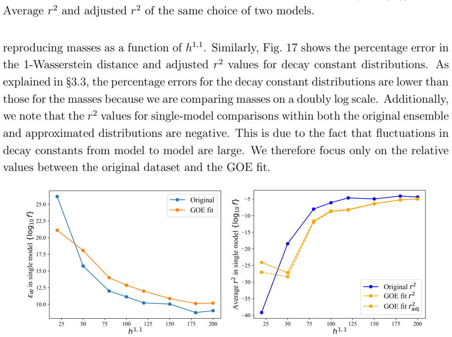
- Predictions of the model become more trustworthy at large $h^{1,1}$, since both the Wasserstein error and the adjusted $r^2$ values improve as the number of axions grows.
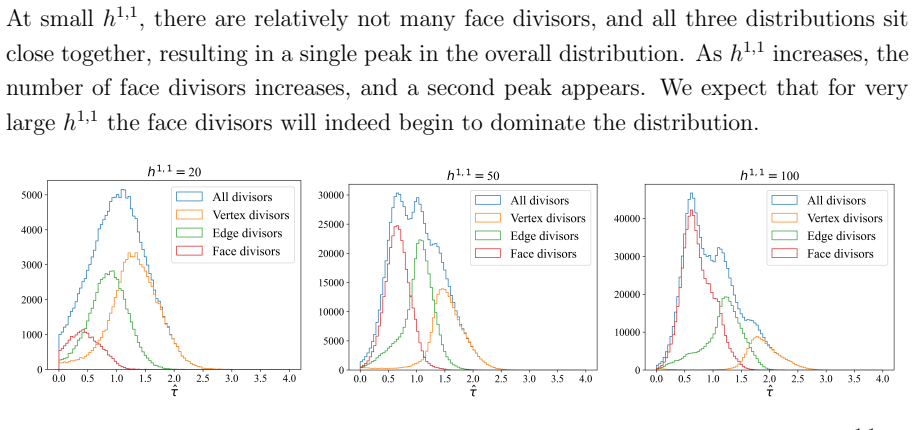
- The decomposition into vertex, edge, and face divisors explains the second peak that appears in the overall volume distribution at moderate $h^{1,1}$ and predicts that face divisors dominate at very large $h^{1,1}$.
- Because the model depends only on divisor volumes and neglects instanton charge structure, it implies that the broad statistical features of the axiverse are insensitive to the detailed charge lattice of each compactification.
Reading between the lines
- If the universality extends beyond toric hypersurfaces, the same GOE ansatz makes a sharp, testable prediction for the normalized divisor-volume spectra of other Calabi-Yau constructions such as complete-intersection Calabi-Yau threefolds or Calabi-Yau fourfolds, which the paper lists as future directions.
- The paper samples one triangulation per polytope and uses random-walk endpoints rather than a Weil-Petersson-weighted measure; a natural check is whether the fitted parameters $(a,b,c)$ drift under those alternative measures while the same level-spacing shape survives, which would identify the universal shape, not the mean growth, as the robust content.
- The model could be inverted phenomenologically: given an observed axion mass or decay-constant distribution, one could fit $(a,b,c)$ and read off an effective number of axions $h^{1,1}$, turning axion experiments into a probe of landscape statistics.
- The GOE level-spacing form suggests that divisor volumes behave like eigenvalue spacings with level repulsion; an explicit test is whether the empirical $p(\hat\tau)$ approaches zero as $\hat\tau \to 0$ in datasets generated with different sampling measures, and whether the three sub-distributions (vertex, edge, face) each show the same repulsion.
Editorial analysis
A structured set of objections, weighed in public.
Referee Report
Summary. The paper studies divisor-volume statistics in toric hypersurface Calabi-Yau threefolds from the Kreuzer-Skarke database. It claims that suitably normalized vertex, edge, and face divisor volumes have universal distributions across the landscape, that axion masses, decay constants, and the stringy QCD theta-angle can be approximated from divisor volumes alone via Eqs. (3.16) and (3.20), and that a three-piece surrogate model—the GOE level-spacing PDF (5.5), the fitted mean (5.6), and the reconstruction rule (5.7)—can reproduce axion observables across the Kreuzer-Skarke axiverse. The paper is explicit about the construction of its ensemble and about the approximations it makes, and it reports Wasserstein distances and adjusted r^2 values for the comparisons.
Significance. If established, the claimed universality and the surrogate model would be valuable: full geometric scans of axion effective theories could be replaced by a nearly instantaneous statistical model, and the apparent GOE connection would be a striking structural hint about Calabi-Yau geometry. The paper is also commendably transparent about the limitations of its sampling protocol. However, the central evidence is currently in-sample: the GOE shape was selected as the best fit to the same ensemble, the parameters (a,b,c) in (5.6) were fitted to that ensemble, and the approximations (3.16)/(3.20) were validated against exact computations in that same ensemble. The load-bearing premise that the ensemble fairly represents the full landscape is acknowledged by the authors to be questionable. The result is therefore a defensible but not yet fully supported claim of landscape-level universality.
major comments (4)
- [Sec. 3.1] The universeality claim of Sec. 4 and the fitted parameters in Eq. (5.6) rest on the representativeness of the ensemble constructed in Sec. 3.1: one random triangulation per polytope via a random walk in the extended Kaehler cone, and one random point in Kaehler moduli space per geometry. The authors themselves state that "our dataset may not be a fair sample of Calabi-Yau threefolds." The comparison with the exhaustive h^{1,1}<=7 FRST list is a good idea, but it is only described qualitatively and it does not test the high-h^{1,1} regime where the face-divisor second peak drives the model's h^{1,1} dependence. Please provide a quantitative validation on an independent or differently weighted sample—for example, multiple triangulations per polytope, an alternative sampling algorithm, or the exhaustive small-h^{1,1} set—and show that the universal distributions and the parameters (a,b,c) are robust under that change.
- [Secs. 3.3 and 5.2] The "reproduction" of axion observables in Figs. 14-19 is an in-sample consistency check rather than a predictive test. The GOE distribution was selected as the best fit to the same ensemble; (a,b,c) in Eq. (5.6) were fitted to the mean log divisor volume of that ensemble; and the approximations (3.16) and (3.20) were validated against exact computations in that same ensemble. Consequently, the reported Wasserstein distances and adjusted r^2 values measure self-consistency. Please add an out-of-sample test, such as a train/test split of polytopes or h^{1,1} values, or a prediction against the independent exhaustive h^{1,1}<=7 dataset, and report predictive performance.
- [Sec. 5.1] The choice of the GOE level-spacing PDF as the analytic model is not falsifiable as presented because no candidate distributions or their fit statistics are shown. The text says that "a range of candidate analytic probability distributions" was explored, but the reader cannot check whether the GOE choice was strongly favored or only marginally better. Please list the candidate families with their 1-Wasserstein and adjusted-r^2 values, and give the comparison for the separately modeled vertex/edge/face version, for which the text reports lower epsilon_W but worse adjusted r^2.
- [Sec. 4 and Figs. 6-9] The pairwise 1-Wasserstein distances support "universality" only if they are interpreted against a meaningful null model. The normalization in Eq. (4.1) forces each model's mean normalized log volume to unity, which removes an overall scale and reduces the distance between any two models. Please compare the observed pairwise distances with distances between random draws from a fitted null distribution, and report confidence intervals or error bars on the pairwise distances, so that the claim of universality is a quantitative statement rather than a visual one.
minor comments (8)
- [Sec. 1] Typo: "ubiquitious" should be "ubiquitous."
- [Sec. 2.3] Typo: "problen" should be "problem."
- [Sec. 3.1] There is an apparent typo in the reference to the algorithms: the text mentions "Algorithm 1 and Algorithm 23," which should presumably be "Algorithm 1 and Algorithm 2."
- [Eq. (3.6)] The definition of mean(X,Y) in Eq. (3.6) should be made explicit; it is not clear whether it is the arithmetic mean of the pooled sample or the average of the two sample means.
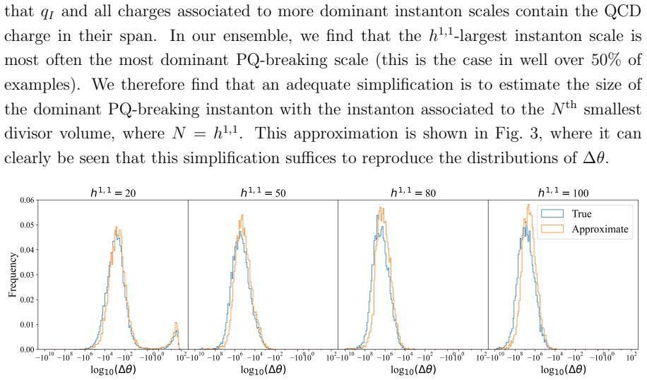
- [Sec. 3.3] The phrase "the h^{1,1}-largest instanton scale is most often the most dominant PQ-breaking scale" is ambiguous; it should say "the h^{1,1}-th largest Lambda_I" or "the instanton associated with the h^{1,1}-th smallest divisor volume."
- [Fig. 11 caption] Typo: "h1.1" should be "h^{1,1}" in the caption.
- [Eq. (5.6)] The fitted parameters in Eq. (5.6), a=3.433, b=5.404, c=4.050, are quoted without uncertainties; please report standard errors or confidence intervals.
- [Sec. 3.1] The claimed match between the ensemble and the exhaustive h^{1,1}<=7 list is not shown quantitatively anywhere; please include a figure or a table with the comparison statistics.
Circularity Check
Section 5's 'reproductions' are in-sample: the GOE shape and the fitted mean (5.6) are both calibrated on the same ensemble that is later used to validate the reconstructed axion observables, so the agreement is a consistency check rather than an independent prediction.
-
fitted input called prediction
[§5.1, Eq. (5.6), and §5.2, Figs. 14–19]
"We fit this trend as ⟨log(τ⃗)⟩fit = a − b × (log10 h1,1)−c, where a ≈ 3.433, b ≈ 5.404, and c ≈ 4.050 are fit parameters. ... Again, we assess the quality of the model by computing ϵW for individual models in our ensemble compared to divisor volume distributions reconstructed using (5.7). ... The trend indicates that the model performs better at reproducing masses as a function of h1,1. ... Finally, we compute ϵW for the distributions of ∆θ compared with the actual values in the explicit ensemble as before."
The parameters (a,b,c) in (5.6) and the GOE shape in (5.5) are both selected by fitting the explicit ensemble: (a,b,c) are fit to ⟨log τ⟩X from that ensemble, and the GOE PDF was adopted because it best matched the τ̂ distributions of that same ensemble. The model (5.7) is then validated by comparing reconstructed divisor volumes, masses, decay constants, and Δθ back to the explicit ensemble. This makes the reported Wasserstein distances and adjusted r2 values in-sample consistency measures, not independent predictions or reproductions. The word 'reproduce' overstates the strength of evidence, since no held-out data or external benchmark is used in the model validation.
full rationale
The paper's geometric content is not definitionally circular. The approximations (3.16) and (3.20) are derived from explicit geometric reasoning and are compared against exact computations of masses and decay constants in the same ensemble; that comparison tests the approximations themselves, independently of the §5 model. Likewise, the §4 universality comparisons of normalized vertex, edge, and face divisor volumes between different geometries are empirical pattern-finding within the ensemble; the normalization (2.6) does force the mean of τ̂ to be 1, but the shape comparisons in Figs. 6–9 contain independent information. The circularity is concentrated in §5: both the analytic distribution (5.5) and the fitted mean (5.6) are calibrated on the same explicit ensemble used to evaluate the model, and the resulting agreement for masses, decay constants, and Δθ is therefore an in-sample check rather than a true reproduction across the landscape. The exhaustive h1,1 ≤ 7 comparison from [24] is a real external anchor, though [24] includes the current author Gendler, and the authors themselves caution that 'our dataset may not be a fair sample of Calabi-Yau threefolds'; that caveat is a limitation on generalization rather than a definitional circularity. Overall, the central derivation chain remains partially circular because the model's predictive claim is tested on its own fitting data, but the underlying geometric approximations and universality observations are not reduced to their inputs by construction.
Assumptions & free parameters
free parameters (3)
- a (fit parameter in Eq. 5.6) =
3.433
- b (fit parameter in Eq. 5.6) =
5.404
- c (fit parameter in Eq. 5.6) =
4.050
assumptions (5)
- standard math Batyrev construction: smooth toric hypersurface Calabi-Yau threefolds correspond to fine, regular, star triangulations of reflexive 4-polytopes.
- domain assumption The orientifold projects out no Kähler moduli and saxions can be stabilized at a dense set of generic points in the Kähler cone.
- domain assumption Prime toric divisors suffice to capture axion physics; autochthonous and non-calibrated divisors are neglected.
- domain assumption The sampled polytopes, triangulations, and moduli points represent the full KS landscape.
- domain assumption For the volume-only approximations, the triple intersection matrix is treated as effectively diagonal and the largest Kähler parameter dominates the total volume.
Cite this review
Pith. "Pith review of Universality in the Axiverse." pith.science (2026). https://pith.science/paper/IMN4E46U
@misc{pith2026250712516,
  author       = {Pith},
  title        = {Pith review of: Universality in the Axiverse},
  year         = {2026},
  howpublished = {\url{https://pith.science/paper/IMN4E46U}},
  note         = {Machine review of arXiv:2507.12516}
}
read the original abstract
Studies of axion effective theories in the type IIB Calabi-Yau landscape have revealed that hierarchies in cycle volumes drive correlations between axion physics and the number of axions in a given model. We analyze distributions of divisor volumes in toric hypersurface Calabi-Yau threefolds, and provide evidence that aspects of these distributions are universal across this landscape. Furthermore, we show that axion observables in this landscape can be approximated efficiently in terms of only divisor volumes. Finally, we propose a simple model for the spectrum of divisor volumes and use this model to reproduce results on axion masses and decay constants across the Kreuzer-Skarke axiverse.
Figures


Figures from the paper (16 more)





Forward citations
Cited by 9 Pith papers
-
Testing F-theory GUTs with the Axiverse
In F-theory GUTs, non-universal ALPs induced by hypercharge flux satisfy g_aγ/m_a well below the QCD axion prediction when gauge couplings unify near the string scale.
-
Axiverse Lampposts
In a hierarchical multi-axion theory with random couplings, axion field ranges shrink with 1/sqrt(N), generic axion–SM couplings are suppressed, but the QCD axion's coupling is unsuppressed.
-
The String Theory Photoverse
Massless string-theory hidden photons acquire dimension-six dipole couplings to SM fermions with suppression scale Λ = αM_s, converting dipole measurements into constraints on the string scale.
-
Towards a Heterotic Axiverse
Generic heterotic axions are heavier than in type IIB; the Strong CP problem is typically unsolved, and a light fuzzy dark matter axion requires a no-gaugino-condensation anisotropic fibred Calabi-Yau.
-
Quantum Gravity Cutoff from Axions: A Type IIB Landscape Study
The bound Λ_QG ≲ 2π √S f holds for C2 and C4 axions in Type IIB Calabi-Yau compactifications even near Kähler moduli space boundaries where co-scaling fails.
-
Tachyonic Encore: A universal shift of inflationary observables
A light axion spectator induces post-inflation tachyonic phases that produce a nearly scale-invariant boost to the curvature power spectrum and alter key inflationary observables in a largely potential-independent manner.
-
The Atacama Cosmology Telescope: Probing new signatures of ultralight axions with gravitational lensing
New upper limits on ultralight axion dark matter fraction (<1.5% at 10^{-26} eV, <9% at 10^{-25} eV at 95% CL) from combined CMB lensing data, plus marginal 2.1σ preference at 10^{-24.5} eV driven by few points.
-
Constraining F-theory Model Building with QCD Axions
QCD axions constrain F-theory base threefolds to have rigid or flux-rigidified divisors, yielding typical axion masses around 10^{-9} eV and decay constants near 10^{15} GeV in allowed regions.
-
Constraining F-theory Model Building with QCD Axions
F-theory models with the Standard Model spectrum are constrained by QCD axion physics, yielding typical detectable axion masses around 10^{-9} eV and decay constants around 10^{15} GeV in allowed regions.
Reference graph
Works this paper leans on
-
[24]
E. Sheridan, F. Carta, N. Gendler, M. Jain, D. J. E. Marsh, L. McAllister, N. Righi, K. K. Rogers, and A. Schachner, Fuzzy Axions and Associated Relics , arXiv:2412.12012
-
[1]
M. Demirtas, C. Long, L. McAllister, and M. Stillman, The Kreuzer-Skarke Axiverse, JHEP 04 (2020) 138, [ arXiv:1808.01282]
arXiv 2020
-
[2]
M. Demirtas, L. McAllister, and A. Rios-Tascon, Bounding the Kreuzer-Skarke Landscape, Fortsch. Phys. 68 (2020) 2000086, [ arXiv:2008.01730]
arXiv 2020
-
[3]
M. Demirtas, M. Kim, L. McAllister, J. Moritz, and A. Rios-Tascon, Computational Mirror Symmetry , JHEP 01 (2024) 184, [ arXiv:2303.00757]
arXiv 2024
-
[5]
A. Chandra, A. Constantin, C. S. Fraser-Taliente, T. R. Harvey, and A. Lukas, Enumerating Calabi-Yau Manifolds: Placing Bounds on the Number of Diffeomorphism Classes in the Kreuzer-Skarke List , Fortsch. Phys. 72 (2024), no. 5 2300264, [arXiv:2310.05909]
work page Pith review arXiv 2024
-
[6]
N. Gendler, B. Heidenreich, L. McAllister, J. Moritz, and T. Rudelius, Moduli space reconstruction and Weak Gravity, JHEP 12 (2023) 134, [ arXiv:2212.10573]
arXiv 2023
-
[7]
N. MacFadden, A. Schachner, and E. Sheridan, The DNA of Calabi-Yau Hypersurfaces, arXiv:2405.08871
- [8]
Show all 48 references
-
[9]
Moritz, Orientifolding Kreuzer-Skarke, arXiv:2305.06363
J. Moritz, Orientifolding Kreuzer-Skarke, arXiv:2305.06363. 33
-
[10]
Svrcek and E
P. Svrcek and E. Witten, Axions In String Theory , JHEP 06 (2006) 051, [hep-th/0605206]
2006 arXiv
-
[11]
J. P. Conlon, The QCD axion and moduli stabilisation , JHEP 05 (2006) 078, [hep-th/0602233]
2006 arXiv
-
[12]
Arvanitaki, S
A. Arvanitaki, S. Dimopoulos, S. Dubovsky, N. Kaloper, and J. March-Russell, String Axiverse , Phys. Rev. D 81 (2010) 123530, [ arXiv:0905.4720]
2010 arXiv
-
[13]
Kreuzer and H
M. Kreuzer and H. Skarke, Complete classification of reflexive polyhedra in four-dimensions, Adv. Theor. Math. Phys. 4 (2000) 1209–1230, [ hep-th/0002240]
2000 arXiv
-
[14]
V. M. Mehta, M. Demirtas, C. Long, D. J. E. Marsh, L. McAllister, and M. J. Stott, Superradiance in string theory , JCAP 07 (2021) 033, [ arXiv:2103.06812]
2021 arXiv
-
[15]
Gendler, D
N. Gendler, D. J. E. Marsh, L. McAllister, and J. Moritz, Glimmers from the Axiverse, arXiv:2309.13145
-
[16]
Gendler and D
N. Gendler and D. J. E. Marsh, QCD Axion Dark Matter in String Theory: Haloscopes and Helioscopes as Probes of the Landscape , arXiv:2407.07143
-
[17]
Demirtas, N
M. Demirtas, N. Gendler, C. Long, L. McAllister, and J. Moritz, PQ axiverse , JHEP 06 (2023) 092, [ arXiv:2112.04503]
2023 arXiv
-
[18]
J. N. Benabou, K. Fraser, M. Reig, and B. R. Safdi, String Theory and Grand Unification Suggest a Sub-Microelectronvolt QCD Axion , arXiv:2505.15884
-
[19]
Halverson, C
J. Halverson, C. Long, B. Nelson, and G. Salinas, Towards string theory expectations for photon couplings to axionlike particles , Phys. Rev. D 100 (2019), no. 10 106010, [ arXiv:1909.05257]
2019 arXiv
-
[20]
Halverson, C
J. Halverson, C. Long, B. Nelson, and G. Salinas, Axion reheating in the string landscape, Phys. Rev. D 99 (2019), no. 8 086014, [ arXiv:1903.04495]
2019 arXiv
-
[21]
V. V. Batyrev, Dual polyhedra and mirror symmetry for calabi-yau hypersurfaces in toric varieties , 1993
1993
-
[22]
A. P. Braun, C. Long, L. McAllister, M. Stillman, and B. Sung, The Hodge Numbers of Divisors of Calabi-Yau Threefold Hypersurfaces , arXiv:1712.04946
-
[23]
Gendler, E
N. Gendler, E. Sheridan, M. Stillman, and D. Wu, Holes in Calabi-Yau Effective Cones, to appear , . 34
-
[25]
Kachru, R
S. Kachru, R. Kallosh, A. D. Linde, and S. P. Trivedi, De Sitter vacua in string theory, Phys. Rev. D 68 (2003) 046005, [ hep-th/0301240]
2003 arXiv
-
[26]
Gendler, O
N. Gendler, O. Janssen, M. Kleban, J. La Madrid, and V. M. Mehta, Axion minima in string theory , arXiv:2309.01831
-
[27]
Bousso, B
R. Bousso, B. Freivogel, and I.-S. Yang, Properties of the scale factor measure , Phys. Rev. D 79 (2009) 063513, [ arXiv:0808.3770]
2009 arXiv
-
[28]
Demirtas, M
M. Demirtas, M. Kim, L. McAllister, J. Moritz, and A. Rios-Tascon, Small cosmological constants in string theory , JHEP 12 (2021) 136, [ arXiv:2107.09064]
2021 arXiv
-
[29]
Rajaguru, A
M. Rajaguru, A. Sengupta, and T. Wrase, Fully stabilized Minkowski vacua in the 26 Landau-Ginzburg model, JHEP 10 (2024) 095, [ arXiv:2407.16756]
2024 arXiv
-
[30]
Gendler, N
N. Gendler, N. MacFadden, L. McAllister, J. Moritz, R. Nally, A. Schachner, and M. Stillman, Counting Calabi-Yau Threefolds, arXiv preprint arXiv:2310.06820 (2023)
2023 arXiv
-
[31]
J. H. T. Yip, C. Arnal, F. Charton, and G. Shiu, Transforming Calabi-Yau Constructions: Generating New Calabi-Yau Manifolds with Transformers , arXiv:2507.03732
-
[32]
Heyes, M
E. Heyes, M. Jain, D. J. Marsh, K. Rogers, A. Schachner, and E. Sheridan, Towards a pipeline through the landscape, to appear ,
-
[33]
Monge, M´ emoiresur la th´ eoriedes d´ eblaiset des remblais
G. Monge, M´ emoiresur la th´ eoriedes d´ eblaiset des remblais. Histoire de l’Acad´ emie Royale des Sciences de Paris, 1781. Reprinted in Oeuvres de Monge, Vol. 1, pp. 666–704, 1896
-
[34]
L. V. Kantorovich, On the translocation of masses , Doklady Akademii Nauk 37 (1942) 199–201. In Russian. English translation in *Management Science*, 5(1), 1958, pp. 1–4
1942
-
[35]
S. S. Vallender, Calculation of the wasserstein distance between probability distributions on the line , Theory of Probability & Its Applications 18 (1974), no. 4 784–786
1974
-
[36]
C. Long, M. Montero, C. Vafa, and I. Valenzuela, The desert and the swampland , JHEP 03 (2023) 109, [ arXiv:2112.11467]. 35
2023 arXiv
-
[37]
4 790–798
Wigner, Eugene P., On the statistical distribution of the widths and spacings of nuclear resonance levels, Mathematical Proceedings of the Cambridge Philosophical Society 47 (1951), no. 4 790–798
1951
-
[38]
Afkhami-Jeddi, A
N. Afkhami-Jeddi, A. Ashmore, and C. Cordova, Calabi-Yau CFTs and random matrices, JHEP 02 (2022) 021, [ arXiv:2107.11461]
2022 arXiv
-
[39]
Ferrari, S
F. Ferrari, S. Klevtsov, and S. Zelditch, Random geometry, quantum gravity and the K¨ ahler potential, Phys. Lett. B 705 (2011) 375–378, [ arXiv:1107.4022]
2011 arXiv
-
[40]
C. Long, L. McAllister, and P. McGuirk, Heavy Tails in Calabi-Yau Moduli Spaces , JHEP 10 (2014) 187, [ arXiv:1407.0709]
2014 arXiv
-
[41]
T. C. Bachlechner, On Gaussian Random Supergravity , JHEP 04 (2014) 054, [arXiv:1401.6187]
2014 arXiv
-
[42]
T. C. Bachlechner, K. Eckerle, O. Janssen, and M. Kleban, The Axidental Universe, JCAP 03 (2025) 050, [ arXiv:1902.05952]
2025 arXiv
-
[43]
Marsh, L
D. Marsh, L. McAllister, and T. Wrase, The Wasteland of Random Supergravities , JHEP 03 (2012) 102, [ arXiv:1112.3034]
2012 arXiv
-
[44]
Dijkgraaf and C
R. Dijkgraaf and C. Vafa, Matrix models, topological strings, and supersymmetric gauge theories, Nucl. Phys. B 644 (2002) 3–20, [ hep-th/0206255]
2002 arXiv
-
[45]
Easther and L
R. Easther and L. McAllister, Random matrices and the spectrum of N-flation , JCAP 05 (2006) 018, [ hep-th/0512102]
2006 arXiv
-
[46]
Di Francesco, P
P. Di Francesco, P. H. Ginsparg, and J. Zinn-Justin, 2-D Gravity and random matrices, Phys. Rept. 254 (1995) 1–133, [ hep-th/9306153]
1995 arXiv
-
[47]
M. R. Douglas, The Statistics of string / M theory vacua , JHEP 05 (2003) 046, [hep-th/0303194]
2003 arXiv
-
[48]
Denef and M
F. Denef and M. R. Douglas, Distributions of flux vacua , JHEP 05 (2004) 072, [hep-th/0404116]
2004 arXiv
-
[49]
Balasubramanian, P
V. Balasubramanian, P. Berglund, J. P. Conlon, and F. Quevedo, Systematics of moduli stabilisation in Calabi-Yau flux compactifications , JHEP 03 (2005) 007, [hep-th/0502058]. 36
2005 arXiv
Reviewed August 6, 2026 · model on record in the stance chip above.
Discussion (0). Sign in to comment.