REVIEW 3 major objections 5 minor 1 cited by
Proton timing bias in Nab silicon detectors is shown to stay below the experiment's 0.3 ns requirement.
Reviewed by Pith at T0; open to challenge. T0 means a machine referee read the full paper against a public rubric. the ladder, T0–T4 →
T0 review · deepseek-v4-flash
2026-08-03 21:14 UTC pith:IO4PAZ27
load-bearing objection Energy and stability characterization for Nab detectors is solid; the sub-0.3 ns proton timing systematic rests on an electron-calibrated simulation not validated against measured proton waveforms. the 3 major comments →
Characterization of Low-energy Ionization Signals in Silicon Detectors for the Nab Experiment
The pith
A machine-rendered reading of the paper's core claim, the machinery that carries it, and where it could break.
Core claim
The paper claims that the pulse-shape systematic in proton time-of-flight measurements for the Nab experiment can be predicted and bounded below 0.3 ns. It achieves this by measuring electron rise times from two radioactive sources on five pixels, fitting a radial impurity-density profile from (2±2)×10^9 cm^-3 at center to (26±2)×10^9 cm^-3 at edge, and applying a drift-velocity scaling factor of 0.979±0.002 to match the electron data. The calibrated simulator is then used to generate 30 keV proton pulses and extract proton timing offsets relative to electrons. The accompanying measurements show a dead layer of (55±2) nm hard or (60±2) nm soft, and no significant proton-peak drift over one y
What carries the argument
The load-bearing tool is NESSE, a pulse-shape simulator named in the paper, which computes induced currents via the Shockley-Ramo theorem using drift trajectories set by the electric field, impurity density, and temperature. The critical step is calibrating this simulator against measured electron rise-time distributions—by simultaneously fitting pixel-by-pixel impurity densities and a global electron drift-velocity scaling factor (0.979±0.002)—and then applying the same calibrated simulator to 30 keV proton pulses to predict timing offsets. This converts a detector characterization into a timing-bias prediction.
Load-bearing premise
The timing-bias estimate assumes that a pulse-shape simulator, tuned only against electron rise-time data from two calibration sources, predicts proton pulse shapes accurately enough that the residual proton-electron timing-offset difference stays below 0.3 ns.
What would settle it
Measure the rise-time distribution of 30 keV protons with the same detector and readout using a pulsed proton beam whose time structure provides the true start time, then compare the measured proton timing offsets to NESSE predictions; if the simulated and measured offsets differ by more than 0.3 ns relative to electron events, the central claim is falsified.
If this is right
- The 0.3 ns timing-bias requirement for Nab proton time-of-flight is achievable, with timing-offset uncertainties around 0.2 ns at -300 V bias.
- Optimal detector running conditions are near -300 V bias and about 120 K, where pulse rise times are short and leakage-current noise is not limiting.
- The measured radial impurity gradient implies pixel-dependent pulse shapes, and the paper provides the per-pixel impurity map needed to correct or simulate them.
- No significant proton-peak drift across a year of liquid-nitrogen cooling cycles indicates that cryo-pumping surface contamination is not degrading the entrance window under the tested conditions.
- Nearest-neighbor cross-talk below about 1% keeps the proton trigger threshold low enough for 25–35 keV protons.
Where Pith is reading between the lines
- If the electron-calibrated drift model extrapolates faithfully to protons, the same calibration procedure could predict timing biases for other particle types without dedicated proton beam time; a direct measurement of proton pulse rise times with a pulsed beam would test this extrapolation.
- The radial impurity gradient suggests that Nab's offline analysis will need per-pixel timing corrections, and other float-zone silicon detectors facing similar rise-time variation could adopt the same calibration method.
- The stability result was obtained at pressures somewhat higher than Nab's projected ultrahigh vacuum; the lack of observed surface deposits is encouraging but the in-situ UHV case remains to be demonstrated.
- The overall approach—deriving a timing model from rise-time distributions of calibration sources—could transfer to other precision beta-decay experiments using segmented silicon detectors.
Editorial analysis
A structured set of objections, weighed in public.
Referee Report
Summary. This paper characterizes a Nab silicon detector using a dedicated low-energy proton source and radioactive electron sources. The energy calibration combines 109Cd/113Sn peaks with Geant4 modeling of source-foil energy losses and temperature corrections; proton energy spectra at 25/30/35 keV yield a hard/soft dead layer of about 55/60 nm and are stable at the calibration-uncertainty level over a year of cooling cycles. Cross-talk between neighboring pixels is measured to be below ~1%. Pulse-shape analysis fits NESSE simulations to electron rise-time distributions to extract a radial impurity-density profile and a drift-velocity scaling factor, then applies the same simulator to 30 keV proton pulses to estimate timing offsets. The paper claims the resulting proton timing systematic uncertainties are below 0.3 ns, sufficient for Nab.
Significance. If the timing claim holds, this is a valuable detector characterization that directly supports the Nab experiment's sub-nanosecond time-of-flight requirement. The energy and dead-layer results are carefully executed: uncertainties from source-foil thickness fits, temperature corrections, and peak extraction are propagated, the SIMS-based dead-layer model is a genuinely parameter-free cross-check, and the one-year proton-peak stability study addresses an important operational concern. The pulse-shape simulation infrastructure is well motivated and the impurity-density characterization is useful in its own right. However, the proton-timing conclusion is only as strong as the electron-to-proton model transfer, and that transfer is not directly validated in the manuscript.
major comments (3)
- [Sec. VI B 2 / Sec. VI A 2, Fig. 21] The paper's central timing claim rests on NESSE being transferred from electron calibration to proton pulses. The simulator is tuned to 109Cd and 113Sn electron rise-time distributions (Sec. VI A 2), and Fig. 21 then uses the same simulator to report timing offsets for 30 keV protons. No measured proton pulse shape or rise-time distribution is compared with NESSE anywhere in the manuscript, even though 30 keV proton waveforms were recorded at 12 bias voltages (Sec. III D), including on radial pixels. The quoted 0.2 ns uncertainty at -300 V is the spread over simulated events, not an estimate of model error from the electron-to-proton extrapolation. A direct proton-pulse comparison, or an explicit quantified model-uncertainty term, is required before the <0.3 ns conclusion is established.
- [Sec. VI B / Sec. VII] The manuscript describes timing-offset standard deviations as satisfying the Nab 0.3 ns systematic requirement. But the Nab requirement applies to the uncertainty of the correction for the time-of-flight bias, i.e., the difference between electron and proton timing offsets. The per-event spatial spread of simulated t_d values does not by itself bound the systematic error of the mean correction; common-mode model errors shift the mean offset without contributing to that spread. The statement that the timing-bias uncertainty can be reduced to <=0.2 ns is also explicitly conditional on characterizing all pixels and the full electron-energy range, which is not demonstrated in this paper.
- [Sec. VI B 2 / Sec. VII] The beta-decay electron that defines t=0 in Nab has a continuous spectrum up to about 1 MeV, while the timing analysis simulates only 87 keV and 364 keV electrons. The paper itself notes an approximately 2 ns average timing-offset difference between these two energies at -300 V (Figs. 20 and 21). Without an energy-dependent electron timing model validated against data, the 'below 0.3 ns' claim applies only to the discrete simulated cases, not to Nab's full electron acceptance. The final paragraph of Sec. VII defers the full electron-energy assessment, so the abstract's blanket statement overstates what is currently established.
minor comments (5)
- [Abstract vs. Sec. V] The abstract quotes a 0.25 keV calibration uncertainty while the body text (Sec. V A and elsewhere) quotes ~0.2 keV. Please harmonize the value and clarify whether the difference is intentional.
- [Eq. (7)] The fit function in Eq. (7) uses an exponential time constant of 1250 and a sigmoid width parameter f, but the units are not stated. Since these parameters enter the timing-offset extraction, please define them explicitly (e.g., ns).
- [Fig. 18 caption] The x-axis is labeled 'Detector pixel ring' but the mapping from pixel numbers (76, 87, 97, 106, 114) to ring numbers is not given in the caption. Adding the mapping would improve reproducibility.
- [Sec. III D] The proton-bias-scan dataset is listed as 30 keV protons at 12 bias voltages, but the pixels used are not stated. Clarify whether these include the same five radial pixels (76, 87, 97, 106, 114) used for the impurity-density fit, since this is relevant to the direct proton validation suggested above.
- [Various] Typographical issues: 'AD8011 pre-amplifer' (Sec. III A 2), 'T rapezoidal' (Sec. IV heading), and 'Pehlet al.' (Sec. V B) should be corrected.
Circularity Check
No significant circularity: NESSE is calibrated on electron rise times and then applied to proton pulses as a physics extrapolation; the missing direct proton-pulse comparison is a validation gap, not an equation-level circular reduction.
full rationale
The derivation chain is: fit the impurity density and a single electron drift-velocity scaling factor to measured 109Cd/113Sn 10-90% rise-time distributions (Sec. VI A 2, Figs. 16-18); use those parameters in NESSE together with Geant4 energy depositions for 30 keV protons (Sec. VI A 1, Fig. 14); and extract timing offsets t_d using Eq. (7) from simulated pulses (Sec. VI B 2, Figs. 20-21). The proton timing offsets are functions of the fitted parameters, but that is true of any calibrated physics model; they are not the same observable as the fitted electron rise-time means, and the paper nowhere sets t_d(proton) equal by construction to the electron rise-time fit. The reported <0.3 ns is the spread or statistical uncertainty of the simulated timing offsets, not a recovered value of the fitted parameters. The absence of a direct comparison between NESSE and the measured 30 keV proton waveforms mentioned in Sec. III D is a genuine validation gap and a legitimate correctness risk---proton pulses could differ because of dead-layer, weighting-field, or high-density ionization effects---but it is not circularity under the stated rules: no equation in the paper reduces the proton timing prediction to the fitted electron data. The self-citations to NESSE [42] and Ref. [13] are load-bearing for model details, but Ref. [13] is a published, peer-reviewed detector-model paper and the key detector-specific parameters are re-fit here to the authors' own measured data; no uniqueness claim or ansatz is imported as a forced alternative. The energy/dead-layer and proton-peak-stability results are independent of the timing model. Score 0.
Axiom & Free-Parameter Ledger
free parameters (4)
- Drift velocity scaling factor =
0.979 ± 0.002
- Pixel impurity densities (Pixels 76, 87, 97, 106, 114) =
2e9 to 26e9 cm^-3
- Dead layer thickness (hard/soft) =
55 ± 2 nm hard, 60 ± 2 nm soft
- Source foil thicknesses (Mylar, Aluminum) =
6.32 ± 0.88 um, 0.66 ± 0.47 um
axioms (6)
- domain assumption NESSE pulse-shape simulation faithfully represents the Nab detector response, including weighting field, charge drift, and electronics.
- domain assumption Electric field in the detector is given by Eq. (4) with uniform impurity density per pixel.
- domain assumption Drift-velocity data from Canali et al. (Ref. [43]) apply to this silicon at Nab temperatures after a single multiplicative scaling.
- domain assumption Geant4 models of source foils and energy deposition are accurate enough for calibration corrections.
- ad hoc to paper The exponentially modified sigmoid (Eq. 7) extracts t0 without unmodeled bias when applied to simulated and real pulses.
- domain assumption Charge collection efficiency in the dead layer is described by hard or soft dead-layer models.
Cite this review
Pith. "Pith review of Characterization of Low-energy Ionization Signals in Silicon Detectors for the Nab Experiment." pith.science (2026). https://pith.science/paper/IO4PAZ27
@misc{pith2026251115912,
  author       = {Pith},
  title        = {Pith review of: Characterization of Low-energy Ionization Signals in Silicon Detectors for the Nab Experiment},
  year         = {2026},
  howpublished = {\url{https://pith.science/paper/IO4PAZ27}},
  note         = {Machine review of arXiv:2511.15912}
}
read the original abstract
The Nab (Neutron a b) experiment is designed to measure the beta-antineutrino angular correlation in free neutron $\beta$ decay with an ultimate precision goal of 0.1%, providing input for tests of Cabibbo-Kobayashi-Maskawa (CKM) matrix unitarity. This measurement is performed via detection of electrons and protons in delayed coincidence using custom large-area segmented silicon detectors. We present the characterization of one such detector system to establish the proton energy and timing response, using a dedicated proton accelerator. The detected proton peak was studied for 25 keV, 30 keV, and 35 keV incident protons on a set of detector segments and multiple cooling cycles over a one year period. Ionization losses were consistent with models of the detector dead layer with thicknesses less than 100 nm. The detected proton peak was stable within the uncertainty from energy calibration (0.25 keV). The rise times of detector pulses from $^{109}$Cd and $^{113}$Sn conversion electron sources were used to extract the impurity density profile and establish a precise model for the detector timing response. The observed impurity density profile varied from $(2 \pm 2) \times 10^9$ cm$^{-3}$ at the center to $(26 \pm 2) \times 10^9$ cm$^{-3}$ at the edge. This impurity density profile was then used to characterize systematic effects in proton time-of-flight measurements due to detector pulse-shape effects; the resultant proton timing systematic uncertainties were below 0.3 ns, which is sufficient for the Nab experiment.
Figures



Forward citations
Cited by 1 Pith paper
-
Characterisation of a Thick Pixelated Silicon Detector for Electron Spectroscopy of Neutron Beta Decay
A commercial 2 mm pixelated silicon detector achieves about 3-4 keV resolution and high linearity for electron spectroscopy, but percent-level charge sharing must be mitigated before it meets PERC's precision goals.
Reference graph
Works this paper leans on
-
[1]
In our temperature model, we assumed a linear decrease in ionization energy,ϵ ph, as a function of temperature for Si [35]
Temperature Correction In order to analyze the temperature dependence of the Nab detectors, 109Cd data were taken atV b =−300 V for three different temperatures: 124 K, 133 K, and 151 K. In our temperature model, we assumed a linear decrease in ionization energy,ϵ ph, as a function of temperature for Si [35]. A small dependence on the temperature is also ...
-
[2]
transition boards
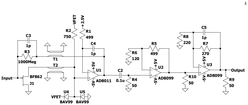
Amplifier and Electronics Each pixel contact on the detector is coupled to a cryogenically-cooled junction field-effect transistor (JFET) in-tandem with a current-feedback amplifier. This configuration acts as a trans-impedance pre- amplifier which precedes two further gain stages. Fig- ure 3 shows the schematic for one pixel’s amplification chain. The BF...
-
[3]
shaping time
Detector Cooling The detector system contains the detector, and front- end amplifiers for each segment, as well as the necessary provisions for cooling (Fig. 2). The detector and JFET were cooled using liquid nitrogen (LN 2), regulated with a mass-flow controller. Cryogenic cooling drastically re- duces the diode-junction leakage current, and also im- pro...
-
[4]
Emitted source electrons have energy dependent losses through the foil that must be accounted for in the energy calibration
Radioactive Source Event Simulation The radioactive source configuration consists of two layers of aluminized Mylar foil that are glued together to encapsulate the radioactive material suspended in a carrier compound. Emitted source electrons have energy dependent losses through the foil that must be accounted for in the energy calibration. To do so, the ...
-
[5]
linear calibration
Energy Loss Correction from Event Simulation We expect energy losses for conversion electrons due to the source configuration and must apply a correction for both 113Sn and 109Cd simultaneously. We expect losses to be significant for the 109Cd conversion lines, as they are much lower in energy compared to the 113Sn lines. We also expect losses to be radia...
-
[6]
After apply- ing all corrections, the linear calibration gain parame- ter changed by<1% for all pixels and the gain uncer- tainty decreased by a factor of∼4 on average
Calibration Results Following the calibration scheme presented in this section, we applied a temperature correction from [35] and an energy-loss correction for each pixel, constructed from the most likely source configuration. After apply- ing all corrections, the linear calibration gain parame- ter changed by<1% for all pixels and the gain uncer- tainty ...
-
[7]
hard” dead layer) or one where, due to dif- fusive processes, partial charge collection occurs (a “soft
Non-linearity from Calibration Results We expect the Si detector system response to be highly linear [35], with our electronics chain evaluated to demon- strate smaller than 0.3% non-linear response in [11], how- ever non-linear effects can arise from charge-trapping in 10 1.645 1.650 1.655 1.660 Gain (ADC keV ) 76 87 97 106 114 Pixel 0.25 0.00 0.25 0.50 ...
-
[8]
float zone
Pulse Shape Simulation The pulse shape is determined by a convolution of the detector system electronics response and the induced cur- rent on the detector pixel contacts. We modeled the elec- tronics response with a SPICE model, as developed in Ref. [13]. The induced current is determined by the pixel weighting field and the electron and hole drift traje...
-
[9]
Pixel ring
Impurity Density Profile Characterization The detector mobilities and pixel impurity densities of the detector were determined by comparing 10-90% rise time distributions between NESSE pulses and pulses from 109Cd and 113Sn sources (described in Sec. IV C). The 113Sn 364 keV and 109Cd 87 keV conversion electron peaks were used in the rise time distributio...
-
[10]
Pulses were simulated for 30 keV protons, 87 keV electrons from a 109Cd source, and 364 keV elec- trons from a 113Sn source as described in Section VI A 1
Detector Timing Bias The expected timing bias was determined by taking simulated electron and proton pulses, adding baseline noise from the corresponding calibration source data, and comparing the extractedt 0 to the simulation start time (tT = 0). Pulses were simulated for 30 keV protons, 87 keV electrons from a 109Cd source, and 364 keV elec- trons from...
2019
-
[11]
V. Cirigliano, A. Crivellin, M. Hoferichter, and M. Moulson, Physics Letters B838, 137748 (2023), arXiv:2208.11707 [hep-ph]
Pith/arXiv arXiv 2023
-
[12]
M. Antonelli, D. M. Asner, D. Bauer, T. T.Becher, 18 M. Beneke, A. J. Bevan, M. Blanke, C. Bloise, M. Bona, A. Bondar, C. Bozzi, J. Brod, A. J. Buras, N. Cabibbo, A. Carbone, G. Cavoto, V. Cirigliano, M. Ciuchini, J. P. Coleman, D. P. Cronin-Hennessy, J. P. Dalseno, C. H. Davies, F. DiLodovico, J. Dingfelder, Z. Dolezal, S. Donati, W. Dungel, G. Eigen, U....
Pith/arXiv arXiv 2010
-
[13]
J. D. Jackson, S. B. Treiman, and H. W. Wyld, Physical Review106, 517 (1957)
1957
-
[14]
Po˘ cani´ c, R
D. Po˘ cani´ c, R. Alarcon, L. Alonzi, S. Baeßler, S. Bal- ascuta, J. Bowman, M. Bychkov, J. Byrne, J. Calarco, V. Cianciolo, and et al., Nuclear Instruments and Meth- ods in Physics Research Section A: Accelerators, Spec- trometers, Detectors and Associated Equipment611, 211–215 (2009)
2009
-
[15]
Baeßler, R
S. Baeßler, R. Alarcon, L. P. Alonzi, S. Balascuta, L. Barr´ on-Palos, J. D. Bowman, M. A. Bychkov, J. Byrne, J. R. Calarco, T. Chupp, T. V. Cianci- olo, C. Crawford, E. Frleˇ z, M. T. Gericke, F. Gl¨ uck, G. L. Greene, R. K. Grzywacz, V. Gudkov, D. Har- rison, F. W. Hersman, T. Ito, M. Makela, J. Martin, P. L. McGaughey, S. McGovern, S. Page, S. I. Pentt...
2013
-
[16]
Baeßler, H
S. Baeßler, H. Acharya, R. Alarcon, L. J. Brous- sard, M. Bowler, D. Bowman, J. H. Choi, L. Christie, T. Chupp, S. Clymer, C. Crawford, G. Dodson, N. Fomin, J. Fry, M. Gericke, R. Godri, F. M. Gonza- lez, G. Greene, A. Hagemeier, J. Hamblen, L. Hayen, C. Hendrus, A. Jezghani, H. Li, N. Macsai, M. Makela, R. Mammei, D. G. Mathews, A. Mendelsohn, P. Mueller...
2024
-
[17]
Urban, M
K. Urban, M. Carminati, M. Descher, F. Edzards, D. Fink, C. Fiorini, M. Gugiatti, D. Hinz, T. Houdy, P. King, P. Lechner, S. Mertens, D. Siegmann, M. Steidl, and J. Wolf, Journal of Instrumentation17(09), C09020
-
[18]
S. Mertens, A. Alborini, K. Altenm¨ uller, T. Bode, L. Bombelli, T. Brunst, M. Carminati, D. Fink, C. Fior- ini, T. Houdy, A. Huber, M. Korzeczek, T. Lasserre, P. Lechner, M. Manotti, I. Peric, D. C. Radford, D. Sieg- mann, M. Slez´ ak, K. Valerius, J. Wolf, and S. W¨ ustling, Journal of Physics G: Nuclear and Particle Physics46, 065203 (2019), arXiv:1810...
Pith/arXiv arXiv 2019
-
[19]
Wietfeldt, G
F. Wietfeldt, G. Darius, M. Dewey, N. Fomin, G. Greene, J. Mulholland, W. Snow, and A. Yue, Physics Procedia 51, 54 (2014), eSS Science Symposium on Neutron Parti- cle Physics at Long Pulse Spallation Sources, NPPatLPS 2013
2014
-
[20]
Salas-Bacci, P
A. Salas-Bacci, P. L. McGaughey, S. Baeßler, L. Brous- sard, M. F. Makela, J. Mirabal, R. W. Pattie, D. Poˇ cani´ c, S. K. Sjue, S. I. Penttila, W. S. Wilburn, A. R. Young, B. A. Zeck, and Z. Wang, Nuclear Instruments and Meth- ods in Physics Research, Section A: Accelerators, Spec- trometers, Detectors and Associated Equipment735, 408 (2014)
2014
-
[21]
L. J. Broussard, B. A. Zeck, E. R. Adamek, S. Baeßler, N. Birge, M. Blatnik, J. D. Bowman, A. E. Brandt, M. Brown, J. Burkhart, N. B. Callahan, S. M. Clay- ton, C. Crawford, C. Cude-Woods, S. Currie, E. B. Dees, X. Ding, N. Fomin, E. Frlez, J. Fry, F. E. Gray, S. Hasan, K. P. Hickerson, J. Hoagland, A. T. Holley, T. M. Ito, A. Klein, H. Li, C. Y. Liu, M. ...
2017
-
[22]
L. J. Broussard, R. Alarcon, S. Baeßler, L. Barr´ on Pa- los, N. Birge, T. Bode, J. D. Bowman, T. Brunst, J. R. Calarco, J. Caylor, T. Chupp, V. Cianciolo, C. Crawford, G. W. Dodson, J. DuBois, W. Fan, W. Farrar, N. Fomin, E. Frleˇ z, J. Fry, M. T. Gericke, F. Gl¨ uck, G. L. Greene, R. K. Grzywacz, V. Gudkov, C. Hendrus, F. W. Hers- man, T. Ito, H. Li, N....
2017
-
[23]
L. Hayen, J. H. Choi, D. Combs, R. J. Taylor, S. Baeßler, N. Birge, L. J. Broussard, C. B. Crawford, N. Fomin, M. Gericke, F. Gonzalez, A. Jezghani, N. Macsai, M. Makela, D. G. Mathews, R. Mammei, M. McCrea, A. Mendelsohn, A. Nelsen, G. Riley, T. Shelton, S. Sjue, E. Smith, A. R. Young, and B. Zeck, Physical Review C 107, 10.1103/PhysRevC.107.065503 (2023)
- [24]
-
[25]
F. M. Gonzalez, J. H. Choi, H. Acharya, S. Cly- 19 mer, A. Hagemeier, D. G. Mathews, A. Mendelsohn, A. Nelsen, H. Rahangdale, L. Richburg, R. Alarcon, A. Atencio, S. Baeßler, T. Bailey, N. Birge, D. Boris- senko, M. Bowler, L. J. Broussard, A. T. Bryant, J. Caylor, T. Chupp, C. Crawford, R. A. Croley, M. Cruz, G. Dodson, W. Fan, D. Fellers, N. Fomin, E. F...
arXiv 2025
-
[26]
J. Fry, R. Alarcon, S. Baessler, S. Balascuta, L. Barron- Palos, T. Bailey, K. Bass, N. Birge, A. Blose, D. Boris- senko, J. D. Bowman, L. J. Broussard, A. T. Bryant, J. Byrne, J. R. Calarco, J. Caylor, K. Chang, T. Chupp, T. V. Cianciolo, C. Crawford, X. Ding, M. Doyle, W. Fan, W. Farrar, N. Fomin, E. Frlez, M. T. Gericke, M. Ger- vais, F. Gluck, G. L. G...
Pith/arXiv arXiv 2019
-
[27]
Micron Semiconductor Ltd, Micron semiconductor ltd
-
[28]
Analog Devices, LTSPICE, https://www.analog.com/en/resources/design-tools- and-calculators/ltspice-simulator.html
-
[29]
Mathews, H
D. Mathews, H. Acharya, C. Crawford, M. Gervais, A. Jezghani, M. McCrea, A. Nelsen, A. Atencio, N. Birge, L. Broussard, J. Choi, F. Gonzalez, H. Li, N. Macsai, A. Mendelsohn, R. Mammei, G. Riley, and R. White- head, Nuclear Instruments and Methods in Physics Re- search Section A: Accelerators, Spectrometers, Detectors and Associated Equipment1071, 170079 (2025)
2025
-
[30]
D. G. Mathews, C. B. Crawford, S. Baeßler, N. Birge, L. J. Broussard, F. Gonzalez, L. Hayen, A. Jezghani, H. Li, R. Mammei, A. Mendelsohn, G. Randall, G. V. Riley, and D. C. Schaper, Journal of Open Source Soft- ware9, 6598 (2024)
2024
-
[31]
G. F. Knoll,Radiation detection and measurement(John Wiley & Sons, Inc, 2024)
2024
-
[32]
Gl¨ uck, Physical Review D47, 2840 (1993)
F. Gl¨ uck, Physical Review D47, 2840 (1993)
1993
-
[33]
R. C. Barber, R. L. Bishop, H. E. Duckworth, J. O. Meredith, F. C. G. Southon, P. Van Rookhuyzen, and P. Williams, Review of Scientific Instruments42, 1 (1971)
1971
-
[34]
Harrison,Low-Energy Proton Accelerator for Detector Testing, M.Sc
D. Harrison,Low-Energy Proton Accelerator for Detector Testing, M.Sc. thesis, University of Manitoba, Winnipeg (2013)
2013
-
[35]
Blachot, Nuclear Data Sheets111, 1497 (2010)
J. Blachot, Nuclear Data Sheets111, 1497 (2010)
2010
-
[36]
Kumar, J
S. Kumar, J. Chen, and F. Kondev, Nuclear Data Sheets 137, 196 (2016)
2016
-
[37]
Eckert & Ziegler Isotope Products, Eckert & Ziegler Ref- erence & Calibration Sources (2007)
2007
-
[38]
V. T. Jordanov and G. F. Knoll, Nuclear Instruments and Methods in Physics Research Section A: Acceler- ators, Spectrometers, Detectors and Associated Equip- ment345, 337 (1994)
1994
-
[39]
Bertuccio and A
G. Bertuccio and A. Pullia, Review of Scientific Instru- ments64, 3294 (1993)
1993
-
[40]
Cornat, 2009 IEEE Sensors , 238–239 (2009)
R. Cornat, 2009 IEEE Sensors , 238–239 (2009)
2009
-
[41]
Pullia, D
A. Pullia, D. Weisshaar, F. Zocca, and D. Bazzacco, IEEE Transactions on Nuclear Science58, 1201 (2011)
2011
-
[42]
Agostinelli, J
S. Agostinelli, J. Allison, K. Amako, J. Apostolakis, H. Araujo, P. Arce, M. Asai, D. Axen, S. Banerjee, G. Barrand, F. Behner, L. Bellagamba, J. Boudreau, L. Broglia, A. Brunengo, H. Burkhardt, S. Chauvie, J. Chuma, R. Chytracek, G. Cooperman, G. Cosmo, P. Degtyarenko, A. Dell’Acqua, G. Depaola, D. Diet- rich, R. Enami, A. Feliciello, C. Ferguson, H. Fes...
2003
-
[43]
Allison, K
J. Allison, K. Amako, J. Apostolakis, H. Araujo, P. Arce Dubois, M. Asai, G. Barrand, R. Capra, S. Chau- vie, R. Chytracek, G. Cirrone, G. Cooperman, G. Cosmo, G. Cuttone, G. Daquino, M. Donszelmann, M. Dres- sel, G. Folger, F. Foppiano, J. Generowicz, V. Grichine, S. Guatelli, P. Gumplinger, A. Heikkinen, I. Hrivna- cova, A. Howard, S. Incerti, V. Ivanch...
2006
-
[44]
Longoria, A
L. Longoria, A. Naboulsi, P. Gray, and T. MacMahon, Nuclear Instruments and Methods in Physics Research Section A: Accelerators, Spectrometers, Detectors and Associated Equipment299, 308 (1990)
1990
-
[45]
R. Pehl, F. Goulding, D. Landis, and M. Lenzlinger, Nu- clear Instruments and Methods59, 45 (1968)
1968
-
[46]
Allison, K
J. Allison, K. Amako, J. Apostolakis, P. Arce, M. Asai, T. Aso, E. Bagli, A. Bagulya, S. Banerjee, G. Bar- rand, B. Beck, A. Bogdanov, D. Brandt, J. Brown, H. Burkhardt, P. Canal, D. Cano-Ott, S. Chauvie, K. Cho, G. Cirrone, G. Cooperman, M. Cort´ es-Giraldo, G. Cosmo, G. Cuttone, G. Depaola, L. Desorgher, X. Dong, A. Dotti, V. Elvira, G. Folger, Z. Fran-...
2016
-
[47]
B. L. Wall, J. F. Amsbaugh, A. Beglarian, T. Bergmann, H. C. Bichsel, L. I. Bodine, N. M. Boyd, T. H. Bur- ritt, Z. Chaoui, T. J. Corona, P. J. Doe, S. Enomoto, F. Harms, G. C. Harper, M. a. Howe, E. L. Martin, D. S. Parno, D. A. Peterson, L. Petzold, P. Renschler, R. G. H. Robertson, J. Schwarz, M. Steidl, T. D. Van Wechel, B. a. Vandevender, S. W¨ ustli...
Pith/arXiv arXiv 2014
-
[48]
Gugiatti, M
M. Gugiatti, M. Biassoni, M. Carminati, O. Cremonesi, C. Fiorini, P. King, P. Lechner, S. Mertens, L. Pagnanini, M. Pavan, and S. Pozzi, Nuclear Instruments and Meth- ods in Physics Research Section A: Accelerators, Spec- trometers, Detectors and Associated Equipment979, 164474 (2020)
2020
-
[49]
Dearnaley, IEEE Transactions on Nuclear Science11, 249 (1964)
G. Dearnaley, IEEE Transactions on Nuclear Science11, 249 (1964)
1964
-
[50]
Czerbinak, Acta Physicae Superficierum2, 111–121 (1990)
J. Czerbinak, Acta Physicae Superficierum2, 111–121 (1990)
1990
-
[51]
D. B. M. Klaassen, Solid State Electronics35(1992)
1992
-
[52]
R. J. Taylor and L. Hayen, Nesse: A python based solid state detector simulation developed for the Nab experi- ment
-
[53]
Canali, C
C. Canali, C. Jacoboni, F. Nava, G. Ottaviani, and A. Alberigi-Quaranta, Physical Review B12, 2265 (1975)
1975
-
[54]
Schr¨ oder, H
W. Schr¨ oder, H. Riemann, and A. L¨ udge, inEncyclope- dia of Materials: Science and Technology(Elsevier Ltd,
-
[55]
Eli Grushka, Analytical Chemistry44, 1733 (1972)
1972
-
[56]
X.-F. Han, X. Liu, S. Nakano, and K. Kakimoto, Journal of Crystal Growth545, 125752 (2020)
2020
-
[57]
A. P. Jezghani, L. J. Broussard, and C. B. Crawford, arXiv:2012.05937 [physics.ins-det] (2020), not published
Pith/arXiv arXiv 2012
discussion (0)
Sign in with ORCID, Apple, or X to comment. Anyone can read and Pith papers without signing in.