REVIEW 2 major objections 5 minor 72 references
Risk Bounds For Distributional Regression
T0 review · 2 major / 5 minor · reviewed 2026-08-15 · deepseek-v4-flash
Pith's one-line read A single projection estimator yields uniform risk bounds for full conditional CDF estimation, matching mean-regression rates under isotonic and trend-filtering constraints.
desk verdict A useful paper with one load-bearing proof gap: the isotonic n^{-2/3} rate does not follow from Eq. (43) as written, though the rest of the framework is plausible and worth engaging. read the letter →
The pith
A machine-rendered reading of the paper's core claim, the machinery that carries it, and where it could break.
The reading
What carries the argument
The load-bearing object is the pointwise projection estimator: $\hat F(t)=\arg\min_{\theta\in K_t}\|w(t)-\theta\|^2$, with $w(t)=(\mathbb{1}\{y_1\le t\},\dots,\mathbb{1}\{y_n\le t\})^\top$. Lemma 1 shows this estimator coincides with the minimizer of the empirical CRPS, so a proper-scoring-rule justification is built in. The convex-case proofs reduce risk to two complexity measures: a local Gaussian complexity for the expected CRPS (Theorem 1), and the local entropy of the difference set $K-K$ for the worst-case MSE (Theorem 2). The non-convex result (Theorem 3) replaces convexity by a peeling argument over annuli of the error, leaving a bound in terms of an entropy integral plus an approximation error $\sup_t \sqrt n \|F^*(t)-G(t)\|_\infty$. These are the mechanisms that carry the argument.
What would settle it
Recompute the local Gaussian complexity of the isotonic cone at radius $\eta = n^{1/6}$: the bound written in the proof is of order $\eta n^{1/4} = n^{5/12}$, which exceeds the $\eta^2 = n^{1/3}$ threshold that Theorem 1 requires, so the quoted $n^{-2/3}$ CRPS rate stands only if a sharper estimate exists.
Extended reading notes
Core claim
The central claim is that the thresholdwise projection estimator—defined for each t as the Euclidean projection of $w(t)=(\mathbb{1}\{y_i\le t\})$ onto $K_t$—is a statistically principled solution to the empirical CRPS minimization problem, and that its risk can be controlled uniformly in t. In the convex case, Theorem 1 bounds the expected average CRPS by $C\eta^2/n$ whenever a local Gaussian complexity condition holds, and Theorem 2 bounds the worst-case MSE by a local entropy integral of $K-K$; both require $F^*(t)$ to lie in $K_t$. From these, isotonic distributional regression achieves $n^{-2/3}$ and trend filtering achieves $V^{2/(2r+1)} n^{-2r/(2r+1)}$ for both CRPS and worst-case MSE, matching mean-estimation rates. For non-convex $K_t$, Theorem 3 trades convexity for an explicit approximation error and still gives a uniform bound, which Corollary 4 converts into a dense-ReLU-network rate of order $(\log n)/n + \phi_n \log^4 n$. The paper also derives faster, near-parametric rates when the true CDF sequence is piecewise constant or its differences are sparse and well separated.
Load-bearing premise
The main guarantees require the true CDF vector $F^*(t)$ to lie exactly inside the constraint set $K_t$ for every threshold t, and the CRPS bounds additionally require the responses to be supported on a common compact set; if the monotonicity or bounded-variation constraint is misspecified, the convex-case rates do not apply.
Editorial extensions
If this is right
- Isotonic distributional regression attains an expected average CRPS of order $n^{-2/3}$ and a worst-case MSE of order $n^{-2/3} + (\log n)/n$, matching the minimax rate for isotonic mean regression.
- Trend-filtering distributional regression attains $V^{2/(2r+1)} n^{-2r/(2r+1)}$ for both metrics, so the total-variation bound $V$ behaves exactly as in univariate trend filtering.
- When the true CDF sequence has few strict increases (isotonic case) or its $r$-th order differences are sparse with separated segments, the bounds improve to nearly parametric rates up to logarithmic factors.
- Dense ReLU network distributional regression achieves the hierarchical-composition rate $\phi_n$ with only log factors, and the guarantee is uniform over all thresholds rather than at a single point.
- The estimator inherits standard algorithms—the pool adjacent violators algorithm for isotonic constraints and trend-filtering solvers for total-variation constraints—so the theoretical rates apply to computationally practical procedures.
Reading between the lines
- Editorial inference: because the CRPS bound integrates squared CDF errors over t, the same projection-plus-local-complexity recipe could produce analogous uniform bounds for other integral scoring rules, such as energy scores with suitable kernels.
- Editorial inference: the isotonic rate $n^{-2/3}$ needs no smoothness or design-density assumptions, so an experimenter can check whether the empirical rate on non-dense covariate grids matches the theory rather than the slower rates that earlier smoothness-based analyses would suggest.
- Editorial inference: the non-convex theorem separates approximation from estimation error, so it likely applies to any constraint class with a known metric entropy, including sparse or additive distributional regression, without new proof machinery.
- Editorial inference: a practical upshot is that shape constraints become essentially free for full-distribution forecasting—users get the same convergence rate they already expect from constrained mean regression.
Signed reviews
Editorial analysis
A structured set of objections, weighed in public.
Referee Report
Summary. The paper proposes a unified projection-based framework for nonparametric distributional regression under structural constraints. For convex constraint sets K_t containing the true CDF evaluation vector F*(t), it derives upper bounds on expected CRPS risk (Theorem 1) and on worst-case MSE uniformly over t (Theorem 2), expressed through local Gaussian complexity and metric entropy integrals. These general results are applied to isotonic regression (Corollary 2, claimed n^{-2/3} rates) and to trend filtering (Corollary 3, claimed V^{2/(2r+1)} n^{-2r/(2r+1)} rates). A third theorem extends the analysis to non-convex and misspecified constraints and is applied to dense ReLU networks (Corollary 4). The paper also contains adaptive-rate refinements for piecewise-constant and sparse-signal cases, and an extensive simulation and real-data study comparing the proposed 'UnifDR' estimators with several benchmarks. All theorems come with proofs in the appendix, and the general convex results are built on a reduction to localized Gaussian complexity in the spirit of prior work on shape-constrained regression.
Significance. If the convex-case results are correct, the paper makes a useful contribution by giving the first uniform-over-t risk guarantees for distributional isotonic regression, trend filtering, and ReLU-network distributional regression, and by showing that the rate for distributional regression can match the corresponding mean-estimation rate. The framework is natural and the proofs are detailed, including the reduction of CRPS estimation to projection estimators. The experiments are comprehensive and consistently favor the proposed methods. However, the flagship isotonic-regression rate in Corollary 2 is not supported by the proof as written: the localized Gaussian complexity bound used there has a scaling inconsistency, so the n^{-2/3} claim currently does not follow from Theorem 1. Since this rate is advertised in the abstract and Section 3.2.1, the issue is load-bearing.
major comments (2)
- [Appendix F.5, Eq. (43); Corollary 2] The proof of Corollary 2 does not establish the claimed n^{-2/3} rate. Equation (43) bounds the local Gaussian complexity by C_1[2 sqrt(2l) eta n^{1/4} + eta^2 / 2^{l-1}]. For a fixed constant l chosen so that the second term is at most eta^2/(2L), the first term is of order C eta n^{1/4}. The text then asserts that with this l one may take eta ~ n^{1/6} to make C eta n^{1/4} <= eta^2/(2L). Direct algebra requires eta >= constant * n^{1/4}; with eta = n^{1/6} the left side is of order n^{5/12} while the right side is of order n^{1/3}, so condition (6) of Theorem 1 fails. With the forced choice eta ~ n^{1/4}, Theorem 1 yields only a CRPS bound of order n^{-1/2}, not the n^{-2/3} stated in (9). A correct localized complexity estimate for the isotonic constraint is needed before the headline rate can be claimed.
- [Appendix F.5, proof of Corollary 2] The reduction to Eq. (43) is not justified: the supremum in condition (6) is over {theta in K_t : ||theta - F*(t)|| <= eta}, and after the substitution u = theta - F*(t) the constraint set is K - F*(t), a shifted version of the isotonic cone, not the cone K itself. The Gaussian-complexity bound for the cone at the origin therefore does not directly control the displayed quantity unless a centering or tangent-cone argument is supplied. Since F*(t) may have strict increases and hence a large tangent cone, this step is load-bearing for the application of Theorem 1.
minor comments (5)
- [Section 2, Notation] There are typos in the notation section: 'Througout' should be 'Throughout', and 'for for eta > 0' should be 'for eta > 0'.
- [Section 3.2.1] The comparison with Mösching and Dümbgen mixes different design assumptions; the sentence 'their covariates are assumed to be asymptotically dense' should state explicitly how the fixed-design spacing affects the comparison, since the claimed rate improvement otherwise appears to compare incomparable settings.
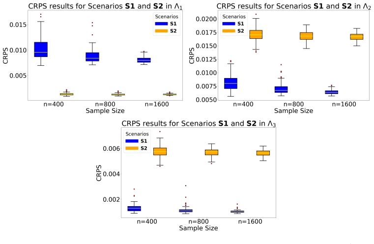
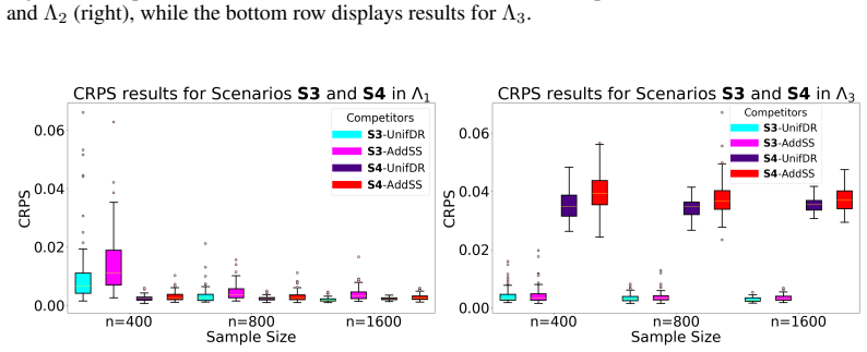
- [Appendix E.2] The heading 'CRPS results on evaluation sets Lambda_1, and Lambda_3, and missing results for S1, S1 and S6 in Lambda_2' contains a typo: 'S1, S1' should read 'S1, S2'.
- [References] Several references are incomplete, for example [4], [12], [13], and [44] lack venue/volume/page details; this makes verification of the cited local-complexity and rate results more difficult.
- [Theorem 3] The notation K(epsilon) = (K-K) cap B_epsilon(0) is introduced in the statement, but the proof writes the entropy integral directly over (K-K) cap B_epsilon(0); please define K(epsilon) once and use it consistently in both the statement and the proof.
Circularity Check
No circular derivation; the risk bounds follow from Gaussian-complexity and metric-entropy reductions, with only minor reliance on self-cited prior lemmas.
full rationale
I walked the derivation chain and found no step where a claimed prediction or first-principles result reduces by construction to its inputs. Theorem 1 reduces the expected CRPS to a local Gaussian complexity condition (6), and Theorem 2 reduces the uniform MSE to a local entropy integral; neither inequality presupposes the n^{-2/3} or V^{2/(2r+1)}n^{-2r/(2r+1)} rates that Corollaries 2 and 3 then derive. The assumption F*(t) in K_t is a modeling assumption, not a fitted parameter renamed as a prediction. The proof of Theorem 1 is actually carried out in Appendix F.2, where a version of Theorem A.1 of Guntuboyina et al. [23] is re-proved, so the main bound does not rest solely on a self-citation. Corollary 2 invokes a Gaussian complexity bound following Chatterjee [13], and Corollary 3 invokes Lemma B.1 of Guntuboyina et al. [23]; these are external published results with independent proofs, and the authors are co-authors of some of them, but the cited lemmas are not the target rates, so the self-citation is not load-bearing in a circular sense. The skeptic's concern about equation (43) in Appendix F.5 is a scaling check that may invalidate the stated proof of Corollary 2, but it is a proof gap or correctness risk, not circularity: the conclusion would fail, rather than be equivalent to an input. Hence the paper is substantially self-contained against external benchmarks, and the only mild reason for a nonzero score is the repeated reliance on the authors' own earlier theorems for key complexity estimates.
Assumptions & free parameters
assumptions (5)
- standard math CRPS is a strictly proper scoring rule (Gneiting and Raftery [22])
- domain assumption The response variables y_i are supported on a common compact set Omega (condition (4))
- domain assumption The true CDF evaluation vector F*(t) belongs to K_t for all t (exact structural constraint)
- ad hoc to paper The local Gaussian complexity condition (6) holds for the constraint sets K_t
- domain assumption For the neural network result, the true regression function G*(.,t) lies in the hierarchical composition class H(l,P) satisfying Assumption 1
Cite this review
Pith. "Pith review of Risk Bounds For Distributional Regression." pith.science (2026). https://pith.science/paper/ISOLEGAR
@misc{pith2026250509075,
  author       = {Pith},
  title        = {Pith review of: Risk Bounds For Distributional Regression},
  year         = {2026},
  howpublished = {\url{https://pith.science/paper/ISOLEGAR}},
  note         = {Machine review of arXiv:2505.09075}
}
read the original abstract
This work examines risk bounds for nonparametric distributional regression estimators. For convex-constrained distributional regression, general upper bounds are established for the continuous ranked probability score (CRPS) and the worst-case mean squared error (MSE) across the domain. These theoretical results are applied to isotonic and trend filtering distributional regression, yielding convergence rates consistent with those for mean estimation. Furthermore, a general upper bound is derived for distributional regression under non-convex constraints, with a specific application to neural network-based estimators. Comprehensive experiments on both simulated and real data validate the theoretical contributions, demonstrating their practical effectiveness.
Figures


Figures from the paper (17 more)




Reference graph
Works this paper leans on
-
[1]
Living on the edge: A geometric theory of phase transitions in convex optimization
Dennis Amelunxen, Martin Lotz, Michael B McCoy, and Joel A Tropp. Living on the edge: A geometric theory of phase transitions in convex optimization. 2013
work page 2013
-
[2]
The isotonic regression problem and its dual.Journal of the American Statistical Association, 67(337):140–147, 1972
Richard E Barlow and Hugh D Brunk. The isotonic regression problem and its dual.Journal of the American Statistical Association, 67(337):140–147, 1972
1972
-
[3]
Richard E Barlow, David J Bartholomew, John M Bremner, and H Dale Brunk.Statistical inference under order restrictions: The theory and application of isotonic regression. Wiley, 1972
work page 1972
-
[4]
On deep learning as a remedy for the curse of dimension- ality in nonparametric regression
Benedikt Bauer and Michael Kohler. On deep learning as a remedy for the curse of dimension- ality in nonparametric regression. 2019
work page 2019
-
[5]
Pierre C Bellec. Sharp oracle inequalities for least squares estimators in shape restricted regression.The Annals of Statistics, 46(2):745–780, 2018
work page 2018
-
[6]
Colin Bennett and Robert C Sharpley.Interpolation of operators. Academic press, 1988
work page 1988
-
[7]
Random forests.Machine learning, 45:5–32, 2001
Leo Breiman. Random forests.Machine learning, 45:5–32, 2001
2001
-
[8]
Leo Breiman, Jerome Friedman, and Charles J Stone. e richard a olshen, 1984
work page 1984
Show all 72 references
-
[9]
University of Missouri-Columbia, 1969
Hugh D Brunk.Estimation of isotonic regression. University of Missouri-Columbia, 1969
1969
-
[10]
Distri- butional random forests: Heterogeneity adjustment and multivariate distributional regression
Domagoj Cevid, Loris Michel, Jeffrey Näf, Peter Bühlmann, and Nicolai Meinshausen. Distri- butional random forests: Heterogeneity adjustment and multivariate distributional regression. Journal of Machine Learning Research, 23(333):1–79, 2022
2022
-
[11]
New risk bounds for 2d total variation denoising
Sabyasachi Chatterjee and Subhajit Goswami. New risk bounds for 2d total variation denoising. IEEE Transactions on Information Theory, 67(6):4060–4091, 2021
2021
-
[12]
On risk bounds in isotonic and other shape restricted regression problems
Sabyasachi Chatterjee, Adityanand Guntuboyina, and Bodhisattva Sen. On risk bounds in isotonic and other shape restricted regression problems. 2015
2015
-
[13]
A new perspective on least squares under convex constraint
Sourav Chatterjee. A new perspective on least squares under convex constraint. 2014
2014
-
[14]
Matrix estimation by universal singular value thresholding
Sourav Chatterjee. Matrix estimation by universal singular value thresholding. 2015
2015
-
[15]
Inference on counterfactual distributions.Econometrica, 81(6):2205–2268, 2013
Victor Chernozhukov, Iván Fernández-Val, and Blaise Melly. Inference on counterfactual distributions.Econometrica, 81(6):2205–2268, 2013
2013
-
[16]
Estimating a distribution function subject to a stochastic order restriction: a comparative study.Journal of Nonparametric Statistics, 24(4):923–933, 2012
Ori Davidov and George Iliopoulos. Estimating a distribution function subject to a stochastic order restriction: a comparative study.Journal of Nonparametric Statistics, 24(4):923–933, 2012
2012
-
[17]
Bayesian density regression.Journal of the Royal Statistical Society Series B: Statistical Methodology, 69(2):163–183, 2007
David B Dunson, Natesh Pillai, and Ju-Hyun Park. Bayesian density regression.Journal of the Royal Statistical Society Series B: Statistical Methodology, 69(2):163–183, 2007
2007
-
[18]
Inferences under a stochastic ordering constraint: the k-sample case.Journal of the American Statistical Association, 100(469):252–261, 2005
Hammou El Barmi and Hari Mukerjee. Inferences under a stochastic ordering constraint: the k-sample case.Journal of the American Statistical Association, 100(469):252–261, 2005
2005
-
[19]
Decomposition methods
Sergio Firpo and Stefanie Sunao. Decomposition methods. InHandbook of Labor, Human Resources and Population Economics, pages 1–32. Springer, 2023
2023
-
[20]
The conditional distribution of excess returns: An empirical analysis.Journal of the American Statistical Association, 90(430):451–466, 1995
Silverio Foresi and Franco Peracchi. The conditional distribution of excess returns: An empirical analysis.Journal of the American Statistical Association, 90(430):451–466, 1995
1995
-
[21]
Multivariate adaptive regression splines.The annals of statistics, 19(1): 1–67, 1991
Jerome H Friedman. Multivariate adaptive regression splines.The annals of statistics, 19(1): 1–67, 1991
1991
-
[22]
Tilmann Gneiting and Adrian E. Raftery. Strictly proper scoring rules, prediction, and estimation. Journal of the American Statistical Association, 102(477):359–378, 2007. 11
2007
-
[23]
Adaptive risk bounds in univariate total variation denoising and trend filtering.The Annals of Statistics, 48:205–229, 2020
Adityanand Guntuboyina, Donovan Lieu, Sabyasachi Chatterjee, and Bodhisattva Sen. Adaptive risk bounds in univariate total variation denoising and trend filtering.The Annals of Statistics, 48:205–229, 2020
2020
-
[24]
Methods for estimating a conditional distribution function.Journal of the American Statistical association, 94(445):154–163, 1999
Peter Hall, Rodney CL Wolff, and Qiwei Yao. Methods for estimating a conditional distribution function.Journal of the American Statistical association, 94(445):154–163, 1999
1999
-
[25]
Some properties of fractional integrals
Godfrey Harold Hardy and John Edensor Littlewood. Some properties of fractional integrals. i. Mathematische Zeitschrift, 27(1):565–606, 1928
1928
-
[26]
Springer, New York, 2nd edition, 2009
Trevor Hastie, Robert Tibshirani, and Jerome Friedman.The Elements of Statistical Learning: Data Mining, Inference, and Prediction. Springer, New York, 2nd edition, 2009. ISBN 978-0387848570
2009
-
[27]
Consistent estimation of distribution functions under increasing concave and convex stochastic ordering.Journal of Business & Economic Statistics, 41(4):1203–1214, 2023
Alexander Henzi. Consistent estimation of distribution functions under increasing concave and convex stochastic ordering.Journal of Business & Economic Statistics, 41(4):1203–1214, 2023
2023
-
[28]
Isotonic distributional regression
Alexander Henzi, Johanna F Ziegel, and Tilmann Gneiting. Isotonic distributional regression. Journal of the Royal Statistical Society Series B: Statistical Methodology, 83(5):963–993, 2021
2021
-
[29]
On models and hypotheses with restricted alternatives.Journal of the American Statistical Association, 60(312):1153–1162, 1965
Robert V Hogg. On models and hypotheses with restricted alternatives.Journal of the American Statistical Association, 60(312):1153–1162, 1965
1965
-
[30]
Optimal rates for total variation denoising
Jan-Christian Hütter and Philippe Rigollet. Optimal rates for total variation denoising. In Conference on Learning Theory, pages 1115–1146. PMLR, 2016
2016
-
[31]
Improving regression performance with distributional losses
Ehsan Imani and Martha White. Improving regression performance with distributional losses. InInternational conference on machine learning, pages 2157–2166. PMLR, 2018
2018
-
[32]
Estimation of distribution functions under second order stochastic dominance.Statistica Sinica, pages 903–926, 2003
Javier Rojo Jiménez and Hammou El Barmi. Estimation of distribution functions under second order stochastic dominance.Statistica Sinica, pages 903–926, 2003
2003
-
[33]
Distributional regression for data analysis.Annual Review of Statistics and Its Application, 11, 2024
Nadja Klein. Distributional regression for data analysis.Annual Review of Statistics and Its Application, 11, 2024
2024
-
[34]
Rage against the mean–a review of distributional regression approaches.Econometrics and Statistics, 26:99–123, 2023
Thomas Kneib, Alexander Silbersdorff, and Benjamin Säfken. Rage against the mean–a review of distributional regression approaches.Econometrics and Statistics, 26:99–123, 2023
2023
-
[35]
Regression quantiles.Econometrica: journal of the Econometric Society, pages 33–50, 1978
Roger Koenker and Gilbert Bassett Jr. Regression quantiles.Econometrica: journal of the Econometric Society, pages 33–50, 1978
1978
-
[36]
Distributional vs
Roger Koenker, Samantha Leorato, and Franco Peracchi. Distributional vs. quantile regression. 2013
2013
-
[37]
On the rate of convergence of fully connected deep neural network regression estimates.The Annals of Statistics, 49(4):2231–2249, 2021
Michael Kohler and Sophie Langer. On the rate of convergence of fully connected deep neural network regression estimates.The Annals of Statistics, 49(4):2231–2249, 2021
2021
-
[38]
A sharp error analysis for the fused lasso, with application to approximate changepoint screening.Advances in neural information processing systems, 30, 2017
Kevin Lin, James L Sharpnack, Alessandro Rinaldo, and Ryan J Tibshirani. A sharp error analysis for the fused lasso, with application to approximate changepoint screening.Advances in neural information processing systems, 30, 2017
2017
-
[39]
An inequality for rearrangements.The American Mathematical Monthly, 60(3):176–179, 1953
Georg Gunther Lorentz. An inequality for rearrangements.The American Mathematical Monthly, 60(3):176–179, 1953
1953
-
[40]
Theoretical analysis of deep neural networks for temporally dependent observations.Advances in Neural Information Processing Systems, 35: 37324–37334, 2022
Mingliang Ma and Abolfazl Safikhani. Theoretical analysis of deep neural networks for temporally dependent observations.Advances in Neural Information Processing Systems, 35: 37324–37334, 2022
2022
-
[41]
Risk bounds for quantile trend filtering
Oscar Hernan Madrid Padilla and Sabyasachi Chatterjee. Risk bounds for quantile trend filtering. Biometrika, 109(3):751–768, 2022
2022
-
[42]
Locally adaptive regression splines.The Annals of Statistics, 25(1):387–413, 1997
Enno Mammen and Sara Van De Geer. Locally adaptive regression splines.The Annals of Statistics, 25(1):387–413, 1997. 12
1997
-
[43]
Scoring rules for continuous probability distributions
James E Matheson and Robert L Winkler. Scoring rules for continuous probability distributions. Management science, 22(10):1087–1096, 1976
1976
-
[44]
Monotone least squares and isotonic quantiles
Alexandre Mösching and Lutz Dümbgen. Monotone least squares and isotonic quantiles. 2020
2020
-
[45]
Sparse spatial autoregressions.Statistics & Probability Letters, 33(3):291–297, 1997
R Kelley Pace and Ronald Barry. Sparse spatial autoregressions.Statistics & Probability Letters, 33(3):291–297, 1997
1997
-
[46]
Temporal-spatial model via trend filtering.arXiv preprint arXiv:2308.16172, 2023
Carlos Misael Madrid Padilla, Oscar Hernan Madrid Padilla, and Daren Wang. Temporal-spatial model via trend filtering.arXiv preprint arXiv:2308.16172, 2023
2023 arXiv
-
[47]
Confidence interval construction and conditional variance estimation with dense relu networks.arXiv preprint arXiv:2412.20355, 2024
Carlos Misael Madrid Padilla, Oscar Hernan Madrid Padilla, Yik Lun Kei, Zhi Zhang, and Yanzhen Chen. Confidence interval construction and conditional variance estimation with dense relu networks.arXiv preprint arXiv:2412.20355, 2024
2024 arXiv
-
[48]
The dfs fused lasso: Linear-time denoising over general graphs.Journal of Machine Learning Research, 18(176):1–36, 2018
Oscar Hernan Madrid Padilla, James Sharpnack, James G Scott, and Ryan J Tibshirani. The dfs fused lasso: Linear-time denoising over general graphs.Journal of Machine Learning Research, 18(176):1–36, 2018
2018
-
[49]
Quantile regression with relu networks: Estimators and minimax rates.Journal of Machine Learning Research, 23(247): 1–42, 2022
Oscar Hernan Madrid Padilla, Wesley Tansey, and Yanzhen Chen. Quantile regression with relu networks: Estimators and minimax rates.Journal of Machine Learning Research, 23(247): 1–42, 2022
2022
-
[50]
On estimating conditional quantiles and distribution functions.Computational statistics & data analysis, 38(4):433–447, 2002
Franco Peracchi. On estimating conditional quantiles and distribution functions.Computational statistics & data analysis, 38(4):433–447, 2002
2002
-
[51]
Order restricted statistical inference/[et al.]
Tim Robertson. Order restricted statistical inference/[et al.]. 1988
1988
-
[52]
Partial distributional policy effects.Econometrica, 80(5):2269–2301, 2012
Christoph Rothe. Partial distributional policy effects.Econometrica, 80(5):2269–2301, 2012
2012
-
[53]
Misspecification testing in a class of conditional distribu- tional models.Journal of the American Statistical Association, 108(501):314–324, 2013
Christoph Rothe and Dominik Wied. Misspecification testing in a class of conditional distribu- tional models.Journal of the American Statistical Association, 108(501):314–324, 2013
2013
-
[54]
Nonlinear total variation based noise removal algorithms.Physica D: nonlinear phenomena, 60(1-4):259–268, 1992
Leonid I Rudin, Stanley Osher, and Emad Fatemi. Nonlinear total variation based noise removal algorithms.Physica D: nonlinear phenomena, 60(1-4):259–268, 1992
1992
-
[55]
Distributional regression forests for probabilistic precipitation forecasting in complex terrain
Lisa Schlosser, Torsten Hothorn, Reto Stauffer, and Achim Zeileis. Distributional regression forests for probabilistic precipitation forecasting in complex terrain. 2019
2019
-
[56]
Nonparametric regression using deep neural networks with relu activation function
Johannes Schmidt-Hieber. Nonparametric regression using deep neural networks with relu activation function. 2020
2020
-
[57]
Springer, 2007
Moshe Shaked and J George Shanthikumar.Stochastic orders. Springer, 2007
2007
-
[58]
Engression: extrapolation through the lens of distribu- tional regression.Journal of the Royal Statistical Society Series B: Statistical Methodology, page qkae108, 2024
Xinwei Shen and Nicolai Meinshausen. Engression: extrapolation through the lens of distribu- tional regression.Journal of the Royal Statistical Society Series B: Statistical Methodology, page qkae108, 2024
2024
-
[59]
Springer Science & Business Media, 2005
Michel Talagrand.The generic chaining: upper and lower bounds of stochastic processes. Springer Science & Business Media, 2005
2005
-
[60]
Maximum-variance total variation denoising for interpretable spatial smoothing
Wesley Tansey, Jesse Thomason, and James Scott. Maximum-variance total variation denoising for interpretable spatial smoothing. InProceedings of the AAAI Conference on Artificial Intelligence, volume 32, 2018
2018
-
[61]
Sparsity and smoothness via the fused lasso.Journal of the Royal Statistical Society: Series B (Statistical Methodology), 67(1):91–108, 2005
Robert Tibshirani, Michael Saunders, Saharon Rosset, Ji Zhu, and Keith Knight. Sparsity and smoothness via the fused lasso.Journal of the Royal Statistical Society: Series B (Statistical Methodology), 67(1):91–108, 2005
2005
-
[62]
Adaptive piecewise polynomial estimation via trend filtering
Ryan J Tibshirani. Adaptive piecewise polynomial estimation via trend filtering. 2014
2014
-
[63]
A primer on bayesian distributional regression.Statistical Modelling, 18(3-4):219–247, 2018
Nikolaus Umlauf and Thomas Kneib. A primer on bayesian distributional regression.Statistical Modelling, 18(3-4):219–247, 2018
2018
-
[64]
Cambridge university press, 2019
Martin J Wainwright.High-dimensional statistics: A non-asymptotic viewpoint, volume 48. Cambridge university press, 2019. 13
2019
-
[65]
Trend filtering on graphs.Journal of Machine Learning Research, 17(105):1–41, 2016
Yu-Xiang Wang, James Sharpnack, Alexander J Smola, and Ryan J Tibshirani. Trend filtering on graphs.Journal of Machine Learning Research, 17(105):1–41, 2016
2016
-
[66]
Non-parametric quantile regression via the k-nn fused lasso.Journal of Machine Learning Research, 22(111):1–38, 2021
Steven Siwei Ye and Oscar Hernan Madrid Padilla. Non-parametric quantile regression via the k-nn fused lasso.Journal of Machine Learning Research, 22(111):1–38, 2021
2021
-
[67]
Dense relu neural networks for temporal-spatial model.arXiv preprint arXiv:2411.09961, 2024
Zhi Zhang, Carlos Misael Madrid Padilla, Xiaokai Luo, Oscar Hernan Madrid Padilla, and Daren Wang. Dense relu neural networks for temporal-spatial model.arXiv preprint arXiv:2411.09961, 2024. 14 A Fast Rates This appendix develops refined risk bounds for distributional regress...
2024 arXiv
-
[68]
16 C Dense ReLU Networks: assumption and definitions In this appendix, we provide additional details for Section 3.3.2
Then sup t∈R nX i=1 1 n bFi(t)−F ∗ i (t) 2 =O P V 2 2r+1 n 2r 2r+1 + logn n ! ,(23) whereV:= sup t∈R pent(F∗(t)). 16 C Dense ReLU Networks: assumption and definitions In this appendix, we provide additional details for Section 3.3.2. Before outlining our assumptions on the fun...
-
[70]
sup θ∈Kt :∥θ−F∗(t)∥≤η g⊤(θ−F ∗(t)) # =E
= Z ∞ 0 P ||bF(t)−F ∗(t)||2 2 >s ds = Z (η+2σ) 2 0 P ||bF(t)−F ∗(t)||2 2 >s ds+ Z ∞ (η+2σ) 2 P ||bF(t)−F ∗(t)||2 2 >s ds =I1 +I 2. To analyze the termI 1 we observe thatP ||bF(t)−F ∗(t)||2 2 >s ≤1, and therefore I1≤(η+ 2σ) 2.(30) For the termI 2, we perform a change of variabl...
-
[71]
Hardy and J.E
Z R |f(t)|2dt= Z ∞ 0 |D(f)(t)| 2dt.(65) 2.[G.H. Hardy and J.E. Littlewood]. Z R |f(t)g(t)|dt≤ Z ∞ 0 D(f)(s)·D(g)(s)ds.(66)
-
[72]
Thenf(t) =D(f)(t)for allt∈[0,∞)
Suppose that f is decreasing and continuous in [0,a) for some a >0 , and f(t) = 0 otherwise. Thenf(t) =D(f)(t)for allt∈[0,∞). Proof. The claim in (65) follows from Proposition 1.8 in Bennett and Sharpley [6]. The inequality in (66) is the well-known G.H Hardy and J.E Littlewoo...
-
[2015]
As before, the spatial domain is discretized into a 100×100 grid, where each grid cell represents an aggregated crime count. The response variable remains the log-transformed total crime counts per grid cell, and grid cells with zero observed crimes are excluded, yielding a fi...
1990
Reviewed August 15, 2026 · model on record in the stance chip above.
Discussion (0). Continue with ORCID to comment.