REVIEW 4 major objections 6 minor 38 references
Estimating Covariance for Global Minimum Variance Portfolio: A Decision-Focused Learning Approach
T0 review · 4 major / 6 minor · reviewed 2026-08-05 · deepseek-v4-flash
Pith's one-line read This paper claims that covariance estimators for minimum-variance portfolios should be trained on the portfolio's own regret loss, and reports lower out-of-sample volatility than standard estimators.
desk verdict A potentially interesting DFL-for-GMVP result whose theory is internally broken and whose baselines need scrutiny. read the letter →
The pith
A machine-rendered reading of the paper's core claim, the machinery that carries it, and where it could break.
The reading
What carries the argument
The machinery is the analytic GMVP map with its exact gradient, combined with a backbone that predicts a positive-semidefinite covariance. The model (DLinear) outputs a lower-triangular matrix $L$, reconstructs $\hat{\Sigma}=LL^\top$, and applies truncated spectral reconstruction (keeping eigenpairs with $\lambda_i \ge \varepsilon\lambda_{\max}$) for inversion stability. The decision loss is the regret between the volatility of the chosen weights and the oracle weights; backpropagation flows through the closed-form solution, and the paper derives the principal-component structure of the resulting gradient in terms of $w$, $\hat{\Sigma}^{-1}w$, and their Kronecker products. These components a
What would settle it
Take any DFL-trained covariance from Section 3.2 and test the assumption $\ker((\hat{\Sigma}^{-1})^2) = \mathrm{span}(\{w, \hat{\Sigma}^{-1}w\})$: because the truncated spectral reconstruction keeps eigenvalues $\lambda_i \ge \varepsilon\lambda_{\max}$, $\hat{\Sigma}$ is positive definite, $(\hat{\Sigma}^{-1})^2$ is invertible, and its kernel is $\{0\}$, not the two-dimensional span. This directly contradicts Proposition 1's condition. For the empirical claim, run the same comparison on a test window outside March 2021-December 2023 (e.g., 2015-2019) and check whether DFL still has lower reali
Extended reading notes
Core claim
The central discovery is that decision-focused learning (DFL) applied to the unconstrained GMVP consistently beats prediction-focused estimation and classical shrinkage in realized volatility. The training objective is the regret loss $L(\theta) = w^*(\hat{\Sigma})^\top \Sigma_{\text{true}} w^*(\hat{\Sigma}) - w^*(\Sigma_{\text{true}})^\top \Sigma_{\text{true}} w^*(\Sigma_{\text{true}})$, and the gradient is decomposed as $dL/d\theta = (dL/dw)(\partial w/\partial \hat{\Sigma})(\partial \hat{\Sigma}/\partial\theta)$, with the weight map given by $w^*(\hat{\Sigma}) = \hat{\Sigma}^{-1}\mathbf{1}/(\mathbf{1}^\top \hat{\Sigma}^{-1}\mathbf{1})$. Propositions 1-3 state that singular vectors of the
Load-bearing premise
The theoretical result assumes certain null spaces of the estimated precision matrix are non-empty and exactly spanned by the portfolio weights and their risk-adjusted counterparts; the paper concedes this may fail in practice, and its own way of making the covariance invertible makes the null spaces empty. Separately, the empirical win assumes a single 2021-2023 test window, without transaction costs, represents how the method would behave generally.
Editorial extensions
If this is right
- Covariance estimators for GMVP should be selected and trained on the regret loss; the paper reports that the decision-focused estimator's out-of-sample annualized volatility is about 0.115-0.138 versus 0.121-0.158 for classical baselines across three equity universes.
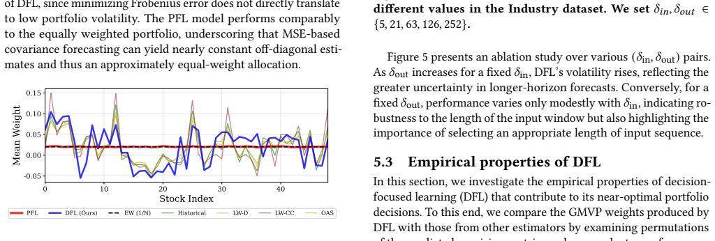
- MSE-trained covariance predictors can collapse toward an equal-weight allocation because they underfit off-diagonal terms, so prediction accuracy is not a proxy for decision quality.
- DFL-trained precision matrices show stable two-block structure, so the estimated weights are more consistent over time than those from the OAS baseline.
- Longer rebalancing horizons raise realized volatility monotonically, which informs how often the portfolio should be rebalanced.
Reading between the lines
- The stated kernel condition behind Propositions 1-3 is likely violated by the paper's own positive-definite covariance reconstruction, as the authors' Remark concedes; that would leave the empirical comparison as the actual support for the contribution (my reading, not the paper's).
- Because the regret loss ignores transaction costs and turnover, the volatility gain may shrink net of costs; adding a turnover penalty to the decision loss is an immediate testable extension.
- The 2021-2023 window features rising rates and elevated volatility; re-running the comparison on calm, low-volatility regimes would tell whether the decision-focused advantage is regime-specific.
- Since only variance is optimized, the method says nothing about returns or Sharpe ratios; combining the decision loss with a return target is the natural next step and the authors list it as future work.
Editorial analysis
A structured set of objections, weighed in public.
Referee Report
Summary. The paper proposes decision-focused learning (DFL) for estimating the covariance matrix used in the unconstrained global minimum-variance portfolio (GMVP). A DLinear network predicts a covariance matrix; GMVP weights are obtained from the closed-form solution; the training loss is the regret loss against the oracle covariance. The paper claims two contributions: (i) a theoretical characterization of the singular vectors / principal components of the decision-gradient (Propositions 1–3), and (ii) an empirical demonstration that DFL portfolios have lower out-of-sample volatility than classical shrinkage estimators and prediction-focused learning across three asset universes and several horizons (Table 1). The empirical section also analyzes the structure of the learned precision matrix, weight stability, and volatility attribution.
Significance. If the empirical result holds, the paper would make a useful practical point: covariance estimators for GMVP can be trained end-to-end on portfolio risk rather than on matrix error. The experimental reporting is mostly honest: five seeds, hyperparameters are listed, early stopping is used, and the comparison includes several standard baselines. The attribution analysis (block structure, low-volatility selection) is a valuable addition. However, the theoretical contribution is not established as stated: the closed-form gradient in Section 3.3 is incorrect, and the kernel assumptions in Proposition 1 are incompatible with the paper's own positive-definite estimator. The empirical comparison is also weakened by unequal information sets between DFL and classical baselines and by the short test window for long horizons. These issues affect the central claims, so the paper needs substantial revision.
major comments (4)
- [Sec. 3.3] The closed-form gradient is incorrect. Direct differentiation of w* = Σ̂^{-1}1/(1^TΣ̂^{-1}1) gives ∂w_i/∂Σ̂_{kl} = -(Σ̂^{-1})_{ik} w_l + D w_i w_k w_l, where D = 1^TΣ̂^{-1}1. Therefore the first term should be -Σ̂^{-1} ⊗ w^T, not -w^T ⊗ (Σ̂^{-1})^T. The paper's expression has the row index attached to the wrong factor: (w^T ⊗ (Σ̂^{-1})^T)_{i,(k,l)} = w_k (Σ̂^{-1})_{l,i}, which is not ∂w_i/∂Σ̂_{kl}. Since Propositions 1–3 analyze this J, their singular-vector conclusions are not derived for the actual problem. If the implementation uses the printed closed form, the reported updates are not gradients of the regret loss; if it uses autodiff through the solve, the theoretical derivation is disconnected. Please correct the formula and re-derive, or state clearly that training differentiates through the solve and remove the closed-form claim.
- [Sec. 3.2 / Prop. 1] The kernel assumptions in Proposition 1 cannot hold for the estimator the paper constructs. Section 3.2 retains eigenpairs with λ_i ≥ ε λ_max, making Σ̂ positive definite for ε>0; hence (Σ̂^{-1})^2 is invertible and its kernel is {0}, not span({w, Σ̂^{-1}w}). Similarly, the second kernel assumption is incompatible with a positive-definite Σ̂. The proof's key step ker(S1) = span({w, Σ̂^{-1}w}) is therefore false. The paper's own Remark concedes that the condition 'may fail in practice.' This makes Propositions 1–3 vacuous as stated. A non-vacuous analysis is needed, for example based on perturbation theory for invertible matrices, or the theoretical contribution should be removed.
- [Table 1 / Sec. 5.1] The comparison between DFL and the classical estimators is not on equal footing. The caption says 'All models use δin = 21 days for estimation,' but the DLinear models are trained on 2010–2018 daily data, whereas Historical, LW-D, LW-CC, and OAS use only the last 21 returns at each rebalance. A 21-day sample covariance is a weak baseline for GMVP; conventional practice often uses longer lookbacks (e.g., 60, 126, or 252 days). Thus the 'consistently superior' claim against classical estimators is not established by Table 1. A fairer comparison would give the classical estimators the same training information (e.g., an expanding window with the same initial training data).
- [Sec. 5.1 / Table 1] The test set spans March 2021 to December 2023, about 2.8 years. For δout = 126 and 252, the number of non-overlapping buy-and-hold rebalances is only about 5 and 2, respectively, so the annualized-volatility estimates in those columns have very large time-series sampling error. No standard errors or significance tests are reported for the volatility differences; the reported standard deviations are over five seeds and do not capture time-series sampling uncertainty. The claim of consistent superiority across horizons in Table 1 is therefore overstated, especially for long horizons.
minor comments (6)
- [Prop. 2 proof] Typo: 'equaiton' should be 'equation'.
- [Sec. 5.2] Typo: 'wherea' should be 'whereas'.
- [Algorithm 1] The subroutine DetectBlocks is called but never defined. Please specify what 'blocks' means and how they are detected.
- [Table 3] The 'average precision' metric is not defined. Please state the formula, how ranks are aggregated over the test period, and how ties are handled.
- [Sec. 3.2] The truncated spectral reconstruction uses a threshold ε, but the value of ε is not reported or included in the hyperparameter tables. Please specify how it is chosen and what values are used.
- [Sec. 4] The phrase 'Σ̂-invariant singular vectors' is used without a formal definition. Please define precisely what invariance means here.
Circularity Check
No circularity in the empirical or theoretical chain; one non-load-bearing self-citation, with correctness risks that are not circularity.
full rationale
The paper's headline claim—DFL yields lower out-of-sample GMVP volatility—is measured on a holdout period with buy-and-hold rebalancing against independent baselines (historical, LW, OAS, PFL); the regret-loss training target uses the training-period true covariance, so the test numbers are not fits relabeled as predictions. The only self-citation ([25], the authors' own MVO-DFL paper) is used to state the gap that DFL has not been applied to GMVP covariance estimation; it is not load-bearing and no uniqueness theorem is imported from it. The theoretical Section 4 is not circular: Propositions 1–3 derive singular-vector structure from explicit kernel/invertibility assumptions rather than from the target conclusion. However, those assumptions are contradicted by the paper's own construction: Section 3.2's truncated spectral reconstruction makes Σ̂ positive definite, so the nontrivial-kernel conditions in Proposition 1 cannot hold; the paper's Remark concedes this. In addition, the closed-form Jacobian in Section 3.3 appears to have transposed Kronecker factors. These are correctness/rigor concerns, not circular steps. The BBC block analysis is a post-hoc descriptive exercise, not a prediction defined by its own output. Overall, no step in the derivation chain reduces to its inputs by construction.
Assumptions & free parameters
free parameters (3)
- Spectral truncation threshold epsilon =
not reported
- Learning rate and batch size (per delta_in, delta_out pair) =
Table 2, e.g., (1e-4, 32)
- Architecture and stopping choices (hidden dim 128, kernel size rule, 50 epochs, patience 7) =
h_dim=128, kernel=max{5,min{delta_in/3,50}}
assumptions (5)
- standard math GMVP closed form w*(Sigma) = Sigma^-1 1 / (1^T Sigma^-1 1)
- domain assumption Realized covariance of the next delta_out days is the ground-truth risk measure (Sigma_true)
- domain assumption Training-period structure (2010-2018) persists into the single test window (2021-2023)
- ad hoc to paper Proposition 1 kernel conditions, e.g., ker((Sigma-hat^-1)^2) = span({w, Sigma-hat^-1 w})
- domain assumption Variance is the decision objective; returns, Sharpe ratio, and costs are out of scope
Cite this review
Pith. "Pith review of Estimating Covariance for Global Minimum Variance Portfolio: A Decision-Focused Learning Approach." pith.science (2026). https://pith.science/paper/IV3XHMLT
@misc{pith2026250810776,
  author       = {Pith},
  title        = {Pith review of: Estimating Covariance for Global Minimum Variance Portfolio: A Decision-Focused Learning Approach},
  year         = {2026},
  howpublished = {\url{https://pith.science/paper/IV3XHMLT}},
  note         = {Machine review of arXiv:2508.10776}
}
read the original abstract
Portfolio optimization constitutes a cornerstone of risk management by quantifying the risk-return trade-off. Since it inherently depends on accurate parameter estimation under conditions of future uncertainty, the selection of appropriate input parameters is critical for effective portfolio construction. However, most conventional statistical estimators and machine learning algorithms determine these parameters by minimizing mean-squared error (MSE), a criterion that can yield suboptimal investment decisions. In this paper, we adopt decision-focused learning (DFL) - an approach that directly optimizes decision quality rather than prediction error such as MSE - to derive the global minimum-variance portfolio (GMVP). Specifically, we theoretically derive the gradient of decision loss using the analytic solution of GMVP and its properties regarding the principal components of itself. Through extensive empirical evaluation, we show that prediction-focused estimation methods may fail to produce optimal allocations in practice, whereas DFL-based methods consistently deliver superior decision performance. Furthermore, we provide a comprehensive analysis of DFL's mechanism in GMVP construction, focusing on its volatility reduction capability, decision-driving features, and estimation characteristics.
Figures


Figures from the paper (9 more)



Reference graph
Works this paper leans on
-
[1]
Akshay Agrawal, Brandon Amos, Shane Barratt, Stephen Boyd, Steven Diamond, and J. Zico Kolter. 2019. Differentiable Convex Optimization Layers. In Advances in Neural Information Processing Systems , Vol. 32
work page 2019
-
[2]
Brandon Amos and J. Zico Kolter. 2017. OptNet: Differentiable Optimization as a Layer in Neural Networks. In Proceedings of the 34th International Conference on Machine Learning (Proceedings of Machine Learning Research, Vol. 70) . PMLR, 136–145
work page 2017
-
[3]
Michael J. Best and Robert R. Grauer. 1991. On the sensitivity of mean-variance- efficient portfolios to changes in asset means: some analytical and computational results. The Review of Financial Studies 4, 2 (April 1991), 315–342
work page 1991
-
[4]
Taras Bodnar, Stepan Mazur, and Yarema Okhrin. 2017. Bayesian estimation of the global minimum variance portfolio. European Journal of Operational Research 256, 1 (Jan. 2017), 292–307
work page 2017
-
[5]
Taras Bodnar, Nestor Parolya, and Wolfgang Schmid. 2018. Estimation of the global minimum variance portfolio in high dimensions. European Journal of Operational Research 266, 1 (April 2018), 371–390
work page 2018
-
[6]
Christian Bongiorno and Damien Challet. 2023. Non-linear shrinkage of the price return covariance matrix is far from optimal for portfolio optimization. Finance Research Letters 52 (2023), 103383
work page 2023
-
[7]
Andrew Butler and Roy H. Kwon. 2023. Integrating Prediction in Mean–Variance Portfolio Optimization. Quantitative Finance 23, 3 (March 2023), 429–452
work page 2023
-
[8]
Zhi Chai, Kai-Kit Wong, Kin-Fai Tong, Yu Chen, and Yangyang Zhang. 2022. Port Selection for Fluid Antenna Systems. IEEE Communications Letters 26, 5 (May 2022), 1180–1184
work page 2022
Show all 38 references
-
[9]
Eldar, and Alfred O
Yilun Chen, Ami Wiesel, Yonina C. Eldar, and Alfred O. Hero III. 2010. Shrink- age Algorithms for MMSE Covariance Estimation. IEEE Transactions on Signal Processing 58, 10 (Oct. 2010), 5016–5029
2010
-
[10]
Chopra and William T
Vijay K. Chopra and William T. Ziemba. 1993. The effect of errors in means, variances and covariances on optimal portfolio choice. Journal of Portfolio Management 19, 2 (1993), 6–11
1993
-
[11]
Tsai-Hsuan Chung, Vahid Rostami, Hamsa Bastani, and Osbert Bastani
-
[12]
Clarke, Harindra De Silva, and Steven Thorley
Roger G. Clarke, Harindra De Silva, and Steven Thorley. 2006. Minimum-variance portfolios in the US equity market. Journal of Portfolio Management 33, 1 (2006), 10–24
2006
-
[13]
Clarke, Harindra De Silva, and Steven Thorley
Roger G. Clarke, Harindra De Silva, and Steven Thorley. 2011. Minimum-variance portfolio composition. Journal of Portfolio Management 37, 2 (2011), 31–45
2011
-
[14]
Giorgio Costa and Garud N. Iyengar. 2023. Distributionally Robust End-to-End Portfolio Construction. Quantitative Finance 23, 10 (Oct. 2023), 1465–1482
2023
-
[15]
Victor DeMiguel, Lorenzo Garlappi, and Raman Uppal. 2009. Optimal versus naive diversification: How inefficient is the 1/N portfolio strategy? The Review of Financial Studies 22, 5 (May 2009), 1915–1953
2009
-
[16]
Predict, then Optimize
Adam N. Elmachtoub and Paul Grigas. 2022. Smart “Predict, then Optimize”. Management Science 68, 1 (Jan. 2022), 9–26
2022
-
[17]
Aaron Ferber, Emily Griffin, Bistra Dilkina, Burcu Keskin, and Meredith Gore
-
[18]
Gabriel Frahm and Christoph Memmel. 2010. Dominating estimators for minimum-variance portfolios. Journal of Econometrics 159, 2 (Dec. 2010), 289– 302
2010
-
[19]
Leonard R. Haff. 1980. Empirical Bayes Estimation of the Multivariate Normal Covariance Matrix. The Annals of Statistics 8, 3 (May 1980), 586–597
1980
-
[20]
Kingma and Jimmy Ba
Diederik P. Kingma and Jimmy Ba. 2014. Adam: A Method for Stochastic Opti- mization. arXiv preprint arXiv:1412.6980 (Dec. 2014). arXiv:1412.6980 [cs.LG]
2014 arXiv
-
[21]
Klein and Vijay S
Robert W. Klein and Vijay S. Bawa. 1976. The effect of estimation risk on optimal portfolio choice. Journal of Financial Economics 3, 3 (June 1976), 215–231
1976
-
[22]
Olivier Ledoit and Michael Wolf. 2003. Improved estimation of the covariance matrix of stock returns with an application to portfolio selection. Journal of Empirical Finance 10, 5 (Dec. 2003), 603–621
2003
-
[23]
Olivier Ledoit and Michael Wolf. 2004. A Well -Conditioned Estimator for Large-Dimensional Covariance Matrices. Journal of Multivariate Analysis 88, 2 (Feb. 2004), 365–411
2004
-
[24]
Olivier Ledoit and Michael Wolf. 2012. Nonlinear Shrinkage Estimation of Large-Dimensional Covariance Matrices. The Annals of Statistics 40, 2 (2012), 1024–1060
2012
-
[25]
Junhyeong Lee, Inwoo Tae, and Yongjae Lee. 2024. Anatomy of Machines for Markowitz: Decision-Focused Learning for Mean-Variance Portfolio Optimiza- tion. arXiv:2409.09684 [q-fin.PM]
2024
-
[26]
Yongjae Lee, Jang Ho Kim, Woo Chang Kim, and Frank J Fabozzi. 2024. An Overview of Machine Learning for Portfolio Optimization. Journal of Portfolio Management 51, 2 (2024)
2024
-
[27]
Jayanta Mandi, Víctor Bucarey, Maxime Mulamba Ke Tchomba, and Tias Guns
-
[28]
Jayanta Mandi, James Kotary, Senne Berden, Maxime Mulamba, Víctor Bucarey, Tias Guns, and Ferdinando Fioretto. 2024. Decision-Focused Learning: Founda- tions, State of the Art, Benchmark and Future Opportunities. Journal of Artificial Intelligence Research 80 (Jan. 2024), 1623–1701
2024
-
[29]
Markowitz
Harry M. Markowitz. 1952. Portfolio selection. Journal of Finance 7, 1 (March 1952), 71–91
1952
-
[30]
In Proceedings of the 39th International Conference on Machine Learning (Proceedings of Machine Learning Research, Vol
Decision-Focused Learning: Through the Lens of Learning to Rank. In Proceedings of the 39th International Conference on Machine Learning (Proceedings of Machine Learning Research, Vol. 162) . PMLR, 14935–14947
-
[31]
Torsten Mörstedt, Bernhard Lutz, and Dirk Neumann. 2024. Cross validation based transfer learning for cross-sectional non-linear shrinkage: A data-driven approach in portfolio optimization. European Journal of Operational Research 318, 2 (May 2024), 670–685
2024
-
[32]
Alessio Petrozziello, Luigi Troiano, Angela Serra, Ivan Jordanov, Giuseppe Storti, Roberto Tagliaferri, and Michele La Rocca. 2022. Deep learning for volatility forecasting in asset management. Soft Computing 26, 17 (Sept. 2022), 8553–8574
2022
-
[33]
Robert C. Merton. 1980. On estimating the expected return on the market: An exploratory investigation. Journal of Financial Economics 8, 4 (Dec. 1980), 323–361
1980
-
[34]
Ailing Zeng, Muxi Chen, Lei Zhang, and Qiang Xu. 2023. Are Transformers Effective for Time Series Forecasting?. InProceedings of the 37th AAAI Conference on Artificial Intelligence, Vol. 37. AAAI Press, 11121–11128. Estimating Covariance for Global Minimum Variance Portfolio: ...
2023
-
[36]
Sanket Shah, Kai Wang, Bryan Wilder, Andrew Perrault, and Milind Tambe
-
[37]
In Advances in Neural Information Processing Systems, Vol
Decision-Focused Learning without Decision-Making: Learning Locally Optimized Decision Losses. In Advances in Neural Information Processing Systems, Vol. 35
-
[2022]
arXiv:2211.08507 [cs.LG]
Decision-Aware Learning for Optimizing Health Supply Chains. arXiv:2211.08507 [cs.LG]
-
[2023]
In Integration of Constraint Programming, Artificial Intelligence, and Operations Research (Lecture Notes in Computer Science)
Predicting Wildlife Trafficking Routes with Differentiable Shortest Paths. In Integration of Constraint Programming, Artificial Intelligence, and Operations Research (Lecture Notes in Computer Science) . Springer Nature Switzerland, 460– 476
Reviewed August 5, 2026 · model on record in the stance chip above.
Discussion (0). Continue with ORCID to comment.