Arctic curve of the free-fermion six-vertex model with reflecting end boundary condition

G.A.P. Ribeiro; I.R. Passos

REVIEW 3 major objections 5 minor 28 references

Arctic curve of the free-fermion six-vertex model with reflecting end boundary condition

T0 review · 3 major / 5 minor · reviewed 2026-08-14 · deepseek-v4-flash

Challenge this review Re-run · record.json Download PDF Read on arXiv ↗ Review JSON

Pith's one-line read The arctic curve of the six-vertex model with reflecting end boundary condition is a unit semicircle centered at (1,1) at the free-fermion point.

desk verdict First analytic arctic curve for reflecting-end six-vertex model at free-fermion point; result is credible and worth refereeing despite a standard-but-unproven tangency assumption. read the letter →

arxiv 1908.05773 v1 pith:J5WA45RL submitted 2019-08-15 math-ph math.MP

I.R. Passos , G.A.P. Ribeiro This is my paper · ORCID

classification math-phmath.MP MSC 82B2082B2382B26

keywords six-vertexmodelreflectingendboundaryconditionarcticcurvefreefermionpointtangentmethodcorrelationsphaseseparationsemicircle

verification ladder T0 review T1 audit T2 compute T3 formal

The pith

A machine-rendered reading of the paper's core claim, the machinery that carries it, and where it could break.

The reading

The paper gives the first analytic derivation of the arctic curve for the six-vertex model with a reflecting end boundary condition, at the free-fermion point Δ=0, μ=0, a=b. On the 2N×N lattice, the curve separating frozen from disordered regions is shown to be a semicircle of unit radius centered at (1,1) in the scaling limit. The derivation feeds the large-N behavior of boundary correlation functions into the Tangent Method, and fixes the contact point with the left boundary at height κ=1. The result fills a gap where only Monte Carlo data existed and agrees with those simulations.

What carries the argument

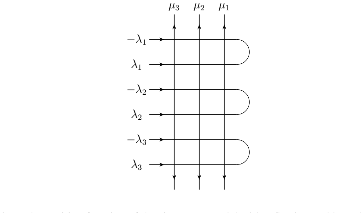
The argument turns on the generating function $h_N(z)=\sum_{r=1}^N H_N^{(r)} z^{r-1}$ for the probability $H_N^{(r)}$ that the unique $c$-vertex in the first column sits in the $r$-th double row. Its large-$N$ logarithm is computed from the free energy, which solves a Liouville equation, giving the function $v(z)$; the Tangent Method then identifies the north-west portion of the arctic curve as the envelope of straight lines whose slope is fixed by $v(z)$ and by a saddle-point condition. The load-bearing geometric input is the tangency assumption that the auxiliary path crosses the left interface as a straight line and then becomes tangent to the curve.

What would settle it

Test the tangency assumption directly: for a moderately large $N$ (say $N=20$ or $30$) at $\Delta=0$, $\mu=0$, $a=b$, sample or exactly enumerate configurations of the extended lattice, locate the boundary of the disordered region, and check whether the separating path is straight up to the interface and tangent to the semicircle $x=1-\cos(2\omega)$, $y=1-\sin(2\omega)$. A systematic kink at the interface, or a boundary location that deviates from $\kappa=1$, would falsify the derived curve.

Watch

Extended reading notes

Core claim

The central claim is that for the six-vertex model with reflecting end boundary condition on a 2N×N lattice, at the free-fermion point (Δ=0, μ=0, a=b), the arctic curve in the thermodynamic limit is the semicircle $x(\omega)=1-\cos(2\omega)$, $y(\omega)=1-\sin(2\omega)$, $\omega\in(-\pi/4,0)$, for the north-west portion, with the south-west portion obtained by $y\to 2-y$; together these form the upper half of the unit circle centered at $(1,1)$. The left-boundary contact point is $\kappa=1$ for every $\lambda$. This is the first analytical determination of the arctic curve for this boundary condition, and it coincides with the west half of the known domain-wall arctic curve on the square lattice.

Load-bearing premise

The derivation assumes that in the scaling limit the auxiliary directed path crosses from the left extension into the main lattice as a straight line and meets the arctic curve tangentially, with no corner at the interface; if it bends there, equations (88)–(89) describe a different curve.

Editorial extensions

If this is right

In the thermodynamic limit the 2N×N reflecting-end lattice splits into two ferroelectric regions (SW and NW) and a central disordered region whose interface is the semicircle.
The left contact point is fixed at height $\kappa=1$, independent of the spectral parameter $\lambda$ at the free-fermion point.
The reflecting-end arctic curve coincides with the west portion of the square-lattice domain-wall arctic curve, so the reflecting boundary does not change the curve shape at this special point.
The asymptotic boundary-correlation function $h_N(z)$ is enough to determine both the contact point and the full parametric curve through the Tangent Method.

Reading between the lines

Editorial extensions of the paper, not claims the author makes directly.

The obstacle the authors identify for $\Delta\neq 0$ and $\mu\neq 0$—the asymmetry between even and odd rows in path weights—could be attacked with a weighted path enumeration on each double row; a successful generalization would place the semicircle result as the free-fermion slice of a larger family of curves.
Since the semicircle is independent of $\lambda$, it provides a parameter-free benchmark for numerical algorithms for reflecting-boundary phase separation.
A direct test of the tangency assumption on finite lattices could be made by measuring the angle of the separating path at the interface; this would separate the geometric assumption from the rest of the saddle-point computation.

Share X Bluesky LinkedIn Reddit HN

Signed reviews

No signed human review yet.

Editorial analysis

A structured set of objections, weighed in public.

Desk editor's note, referee report, and a circularity audit.

Desk Editor's Note

read the letter

Colleague,

Here's my take on 1908.05773. What you should know: this is the first analytic derivation of the arctic curve for the reflecting end boundary condition at Δ=0, and the result is a unit semicircle centered at (1,1), matching the Monte Carlo simulations in [26]. The derivation has no free parameters; the curve is the envelope of straight lines whose slope and intercept are set by the asymptotic of the generating function h_N(z). That asymptotic, Eq. (57), is the real new work, and it comes from a careful determinant-ratio calculation using the authors' earlier boundary correlation results.

What's good: the paper is honest about its scope. It only handles the free-fermion point with a=b and μ=0, and says so plainly in the conclusion. The contact point computation is explicit and gives κ=1 for all λ. The saddle-point machinery is standard and I checked the main equations track. The citation pattern is fine: [23,24] are their own prior work, but those are exactly the results being used as input, not retrofitted.

Soft spots. The Tangency Assumption in Section 4 is the load-bearing geometric input, and it is asserted rather than proved. The stress-test note is correct that if the directed path makes an angle crossing from the left domain into the right domain, the envelope construction would not describe the true arctic curve. I don't think that's a fatal problem here, because this is the same assumption used throughout the Tangent Method literature, and the final curve agrees with independent Monte Carlo evidence. But a referee should ask the authors to state more clearly that this is an assumption inherited from [27], and ideally to discuss why the reflecting boundary does not create a cusp at the interface. The other soft spot is the exponential ansatz for the determinant ratio; it's plausible and consistent, but not fully rigorous. That's typical for this physics literature and shouldn't block publication.

Bottom line: this is a solid, incremental-but-real advance. It extends the known universality of the arctic curve to a new boundary condition and provides the first analytic handle where only numerics existed. I'd bring it to the reading group and I'd cite it if I worked on arctic curves. For peer review: definitely send it out. A serious referee might ask for minor clarifications, but this is not a desk reject.

Referee Report

3 major / 5 minor

Summary. The paper studies the six-vertex model with reflecting end boundary condition on a 2N by N lattice at the free-fermion point Δ=0, μ=0, a=b. It derives the large-N asymptotic behavior of the generating function h_N(z) of boundary correlations by relating it to a ratio of determinants and solving an associated differential equation. It then obtains the contact point of the arctic curve with the left boundary (κ=1) and applies the Tangent Method of Colomo and Sportiello to derive the arctic curve, which is a semicircle centered at (1,1) with unit radius, in agreement with previous Monte Carlo simulations.

Significance. If accepted, this is the first analytical derivation of the arctic curve for the reflecting-end boundary condition, extending the Tangent Method to a model with a reflecting boundary. The main technical contributions are the asymptotic evaluation of the boundary-correlation generating function and the explicit contact-point computation. The paper is clearly written and the main steps are reproducible. However, the derivation is partly heuristic: the exponential ansatz for the determinant ratio and the tangency assumption of the Tangent Method are not proved, and one concavity assertion is incorrect as stated. These points need attention before the result can be considered fully established.

major comments (3)

[Section 4, after Eq. (67)] The derivation of the arctic curve rests on the Tangency Assumption, which is stated rather than proved for the reflecting-end geometry. The paper asserts that the additional path becomes a straight line tangent to the arctic curve and “shall not make an angle” at the interface, but no derivation is given. Equations (88)-(89) and the final semicircle (90) are obtained by taking the envelope of these assumed tangent lines, so this is a load-bearing geometric input. The agreement with Monte Carlo simulations in [26] provides indirect support, but it does not establish the assumption. The authors should either justify the tangency property for this boundary condition or explicitly state that the central result is conditional on this unproven conjecture.
[Section 3.1, Eq. (48)] The exponential ansatz S_N = e^{N\Omega(\mu,\omega)+o(N)}/(N-1)! is assumed without proof. The statement that ~\tau_N behaves similarly to \tau_N because the two determinants differ by one column is only a heuristic. The differential equation (50) is then solved, but the uniqueness of the solution under the boundary condition (46) is not demonstrated. Since the asymptotic (57) that feeds into the Tangent Method is derived from this ansatz, any additional subleading contribution of order N would change the input to the method. The authors should at least verify the ansatz numerically for small N or justify why the o(N) terms cannot affect the exponent.
[Section 4, after Eq. (83)] The claim that H_N^{(r)} assuming values in (0,1] implies its logarithm is concave in \chi is not valid in general; a positive bounded function need not be log-concave. This assertion is used to conclude that the saddle point \chi_0 is a maximum of p(\chi). The authors should provide a direct proof of log-concavity from the explicit determinant representation of H_N^{(r)} or compute p''(\chi_0) explicitly. As written, this step does not rigorously support the saddle-point argument.

minor comments (5)

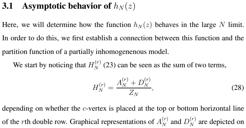
[Eq. (28)] The displayed formula appears to be missing a fraction: it should read H_N^{(r)} = (A_N^{(r)} + D_N^{(r)})/Z_N.
[Eq. (79)] In the last logarithm, the coefficient should be \zeta/(2\chi), not u/(2\chi), to match the factor \ell/(2n-1) in Eq. (77).
[Text after Eq. (79)] The sentence containing “Z_N H_N^{(r)} = A_N^{(r)} + D_N^{(r)} /greaterorsimilar D_N^{(r)}” is garbled; it should read “Z_N H_N^{(r)} = A_N^{(r)} + D_N^{(r)} \geq D_N^{(r)}”.
[Section 4, Eqs. (88)-(90)] The passage from the parametric equations (88)-(89) to the explicit form (90) is not shown. The authors should include the intermediate algebra using the explicit expression for v(z) so that the final semicircle can be verified by the reader.
[Introduction and Conclusion] The paper often refers to the special point as “\Delta=0, \mu=0, a=b”; since in the parametrization (33) this forces \lambda=\pi/4, it would be helpful to state this explicitly in the introduction and conclusion to avoid confusion with the earlier general-\lambda results.

Circularity Check

0 steps flagged · score 0.0 of 10

No significant circularity: the semicircle is derived from independent boundary-correlation asymptotics and the Tangent Method; the Tangency Assumption is an unproven geometric input, not a circular reduction.

full rationale

The derivation chain is self-contained apart from standard citations. The asymptotic input (Eq. 57) is obtained analytically from the partition-function ratio (52) via the free energy (21) and determinant identities (42)-(44); it is fixed before any arctic-curve quantity is computed. The Tangent Method in Sec. 4 then constructs the envelope (88)-(89) from this input and the path enumeration (71), and the final semicircle (90) is solved for, not assumed. The same input independently gives the contact point κ=1. The only load-bearing geometric input is the Tangency Assumption inherited from [27]; the paper states it explicitly rather than smuggling it in, and no equation of the target curve is used to justify it. The comparisons with previous Monte Carlo simulations [26] and with the DWBC west arctic curve [20] are external checks, not inputs. The authors' self-citations [23,24] supply free-energy and correlation results that are parameter-free with stated assumptions and do not contain the target semicircle, so they do not constitute circularity. The Sec. 5 limitations concern generalization to a≠b, Δ≠0, and μ≠0, not a defect in the present derivation.

Assumptions & free parameters 0 free parameters · 5 assumptions · 0 invented entities

The derivation relies on five external ingredients: the Tsuchiya determinant formula, the Liouville free energy, the authors' earlier boundary correlation formulas, an exponential ansatz for the determinant ratio, and the Tangent Method's geometrical assumption. None of these are fitted to the final curve, and none are introduced to force the semicircle.

assumptions (5)

domain assumption Tsuchiya determinant representation of the partition function (Eq. 15).
This representation, derived in [22], is the starting point for computing partition functions and correlations. The paper uses it without re-deriving it.
domain assumption The free energy f(λ,μ) satisfies the Liouville equation and is given by Eq. (21).
From [23], this solution is used in the asymptotic behavior of τ_N and in solving the differential equation for W(μ,ω).
domain assumption The boundary correlation functions used here (Eqs. 22-27) are taken from the authors' previous work [24].
They define G_N^(r), H_N^(r), and the generating function h_N(z) with their determinant and integral representations.
ad hoc to paper The ratio of determinants S_N has the exponential form S_N = e^{NΩ(μ,ω)+o(N)}/(N-1)! (Eq. 48).
This is an ansatz introduced by the authors for the large-N behavior of the determinant ratio. It is plausible because τ_N is known to grow exponentially, but it is not rigorously justified.
domain assumption Tangent Method's Tangency Assumption (Section 4).
The arctic curve is obtained as the envelope of straight lines whose slopes are fixed by the boundary path. This geometrical assumption is taken from [27] and is not proven here.

how reviews work

0 comments

Cite this review

Pith. "Pith review of Arctic curve of the free-fermion six-vertex model with reflecting end boundary condition." pith.science (2026). https://pith.science/paper/J5WA45RL

@misc{pith2026190805773,
  author       = {Pith},
  title        = {Pith review of: Arctic curve of the free-fermion six-vertex model with reflecting end boundary condition},
  year         = {2026},
  howpublished = {\url{https://pith.science/paper/J5WA45RL}},
  note         = {Machine review of arXiv:1908.05773}
}

read the original abstract

We consider the six-vertex model with reflecting end boundary condition. We study the asymptotic behavior of the boundary correlations. This asymptotic behavior is used as an input into the Tangent Method in order to derive analytically the arctic curve at the free fermion point. The obtained curve is a semicircle, which is in agreement with previous Monte Carlo simulations.

Figures

Figures reproduced from arXiv: 1908.05773 by the authors.

**Figure 2.** Partition function of the six-vertex model with re [PITH_FULL_IMAGE:figures/full_fig_p005_2.png] view at source ↗

**Figure 3.** Elements of the K-matrix. as a consequence of the reflection on the left boundary (which reverses the sign of horizontal spectral parameters λ → −λ). Throughout this paper, we denote v±(λ, µ) = v(λ ± µ) where v ∈ {a, b, c}. For the six-vertex model, the Boltzmann weights (1), (2) can be seen as entries of the R-matrix, R(λ) =   a(λ) 0 0 0 0 b(λ) c(λ) 0 0 c(λ) b(λ) 0 0 0 0 a(λ)   , (3) which is a solu… view at source ↗

Figures from the paper (6 more)

**Figure 4.** Figure 4: µ3 µ2 µ1 λ3 −λ3 λ2 −λ2 λ1 −λ1 A (r) N µ3 µ2 µ1 λ3 −λ3 λ2 −λ2 λ1 −λ1 D (r) N [PITH_FULL_IMAGE:figures/full_fig_p011_4.png]

**Figure 5.** Figure 5: In this setting, we define the scaling limit of G (r) N as G(y) = lim r,N→∞ G (r) N , y = lim r,N→∞ 2(N − r) N , y ∈ [0, 2]. (58) Recall the definition of G (r) N is the probability of having a down-arrow between the rth and (r + 1)th double rows. On the other hand, in…

**Figure 5.** Figure 5: Scaling limit of the rectangular lattice and the ex [PITH_FULL_IMAGE:figures/full_fig_p017_5.png]

**Figure 6.** Figure 6: Equivalent way of representing the Boltzmann weig [PITH_FULL_IMAGE:figures/full_fig_p019_6.png]

**Figure 7.** Figure 7: The extended lattice with N = L = 4 and k = 3. top boundaries are fixed, this thick edge originates a directed path that starts one north step before the origin O = (0, 0) and reaches the interface between the two domains at (L, k − 1). As for the domain Λ (r) k , ther…

**Figure 8.** Figure 8: Scaling limit of the extended lattice. Then, the north-west part of arctic curve is the envelope of the family of straight lines Uu(x, y; z) = 0 obtained by varying the parameter of extension of the original lattice, L = uN. The arctic curve parametric coordinates x(z)…

Discussion (0). Continue with ORCID to comment.

Reference graph

Works this paper leans on

28 extracted references · 28 canonical work pages

[26]

Lyberg, V .E

I. Lyberg, V .E. Korepin, G.A.P . Ribeiro, J. Viti, Journ al of Mathematical Physics 59, 053301 (2018)

work page 2018
[27]

Colomo and A

F. Colomo and A. Sportiello, J. Stat. Phys. 164 (2016) 14 88

work page 2016
[1]

Baxter Exactly solved models in statistical mechanics (Academic Press Limited, London, 1982)

R.J. Baxter Exactly solved models in statistical mechanics (Academic Press Limited, London, 1982)

work page 1982
[2]

Korepin, N.M

V .E. Korepin, N.M. Bogoliubov, and A.G. Izergin Quantum inverse scat- tering method and correlation functions (CUP , Cambridge, 1993)

work page 1993
[3]

Kuperberg, Ann

G. Kuperberg, Ann. of Math. (2) 156 (2002) 835

work page 2002
[4]

Bramwell, M.J.P

S.T. Bramwell, M.J.P . Gingras. Science, 294 (2001) 1495

work page 2001
[5]

R.F. Wang, C. Nisoli, R.S. Freitas, J. Li, W. McConville, B.J. Cooley, M.S. Lund, N. Samarth, C. Leighton, V .H. Crespi and P . Schiffer, N ature 439 (2006) 303; N. Rougemaille and B. Canals, Eur. Phys. J. B 92 (2 019) 62; V . Schanilec, Y . Perrin, S. Le Denmat, B. Canals and N. Rougem aille, Ar- tiﬁcial vertex systems by design, arXiv:1902.00452 (2019)

work page Pith review arXiv 2006
[6]

Lieb, Phys

E.H. Lieb, Phys. Rev. Lett. 18 (1967) 692; Phys. Rev. Lett . 18 (1967) 1046; Phys. Rev. Lett. 19 (1967) 108

work page 1967

Show all 28 references

[7]

Brascamp, H

H.J. Brascamp, H. Kunz, F.Y . Wu, J. Math. Phys. 14 (1973) 1 927

1973
[8]

Owczarek and R.J

A.L. Owczarek and R.J. Baxter, J. Phys. A: Math. Gen. 22 (1 989) 1141
[9]

Batchelor, R.J

M.T. Batchelor, R.J. Baxter, M.J. O’Rourke and C.M. Y ung , J. Phys. A: Math. Gen. 28 (1995) 2759. 27

1995
[10]

Korepin and P

V .E. Korepin and P . Zinn-Justin, J. Phys. A 33 (2000) 705 3

2000
[11]

Zinn-Justin, Phys

P . Zinn-Justin, Phys. Rev. E 62 (2000) 3411

2000
[12]

Bleher, V .V

P .M. Bleher, V .V . Fokin, Comm. Math. Phys., 268 (2006) 223; P .M. Bleher, K. Liechty, Comm. Math. Phys. 286 (2009) 777; P .M. Bleher, K. Liechty, J. Stat. Phys. 134 (2009) 463; P .M. Bleher, K. Liechty, Comm. on Pure and Appl. Math., 63 (2010) 779

2006
[13]

Tavares, G.A.P

T.S. Tavares, G.A.P . Ribeiro and V .E. Korepin, J. Stat. Mech. (2015) P06016; T.S. Tavares, G.A.P . Ribeiro and V .E. Korepin, J. Phys. A: Math. Theor. 48 (2015) 454004

2015
[14]

O. Foda, M. Wheeler, J. High Energy Phys., number 7 (2012 ) 186; P . Ble- her, K. Liechty J. Math. Phys. 56 (2015) 023302

2015
[15]

Galleas, J

W. Galleas, J. Lamers, Nucl. Phys. B, 886 (2014) 1003

2014
[16]

Bleher, K

P . Bleher, K. Liechty, Constr Approx (2018) 47: 141

2018
[17]

Korepin, Comm

V .E. Korepin, Comm. Math. Phys., 86 (1982) 391

1982
[18]

Izergin, D.A

A.G. Izergin, D.A. Coker and V .E. Korepin, J. Phys. A: Ma th. Gen. 25 (1992) 4315

1992
[19]

Eloranta, J

K. Eloranta, J. Stat. Phys. 96 (1999) 1091; O.F. Syljuas en and M. B. Zvonarev, Phys. Rev. E, 70 (2004) 016118; D. Allison and N. Re shetikhin, Ann. Inst. Fourier (Grenoble) 55 (2005) 1847

1999
[20]

Colomo, A.G

F. Colomo, A.G. Pronko, J. Stat. Phys. 138 (2010), 662-7 00; F. Colomo, A. G. Pronko, P . Zinn-Justin, J. Stat. Mech.: Theor. Exp. (2010 ) L03002. 28

2010
[21]

Allegra, J

N. Allegra, J. Dubail, J.-M. St´ ephan, and J. Viti, J. St at. Mech., (2016), 053108; J.-M. St´ ephan, J. Stat. Mech., (2017), 103108; L. C ugliandolo, J. Stat. Phys., 167 (2017) 499

2016
[22]

Tsuchiya, J

O. Tsuchiya, J. Math. Phys., 39 (1998) 5946

1998
[23]

Korepin, J

G.A.P Ribeiro and V .E. Korepin, J. Phys. A: Math. Theor. 48 (2015) 045205

2015
[24]

Passos and G.A.P

I.R. Passos and G.A.P . Ribeiro, J. Stat. Mech. (2019) 08 3101

2019
[25]

Cherednik, Theor

I. Cherednik, Theor. Math. Phys. 61 (1984) 977; E.K. Skl yanin, J. Phys. A: Math. Gen. 21 (1988) 2375

1984
[28]

Sylvester, Compt

J.J. Sylvester, Compt. Rend. Acad. Sc. 54 (1862) 129; F. R. Gantmacher The Theory of Matrices, V ol. I (Chelsea Publishing Company, New Y ork, 1959). 29

1959

Pith tools

Reviewed August 14, 2026 · model on record in the stance chip above.

[1] [26]

Lyberg, V .E

I. Lyberg, V .E. Korepin, G.A.P . Ribeiro, J. Viti, Journ al of Mathematical Physics 59, 053301 (2018)

work page 2018

[2] [27]

Colomo and A

F. Colomo and A. Sportiello, J. Stat. Phys. 164 (2016) 14 88

work page 2016

[3] [1]

Baxter Exactly solved models in statistical mechanics (Academic Press Limited, London, 1982)

R.J. Baxter Exactly solved models in statistical mechanics (Academic Press Limited, London, 1982)

work page 1982

[4] [2]

Korepin, N.M

V .E. Korepin, N.M. Bogoliubov, and A.G. Izergin Quantum inverse scat- tering method and correlation functions (CUP , Cambridge, 1993)

work page 1993

[5] [3]

Kuperberg, Ann

G. Kuperberg, Ann. of Math. (2) 156 (2002) 835

work page 2002

[6] [4]

Bramwell, M.J.P

S.T. Bramwell, M.J.P . Gingras. Science, 294 (2001) 1495

work page 2001

[7] [5]

R.F. Wang, C. Nisoli, R.S. Freitas, J. Li, W. McConville, B.J. Cooley, M.S. Lund, N. Samarth, C. Leighton, V .H. Crespi and P . Schiffer, N ature 439 (2006) 303; N. Rougemaille and B. Canals, Eur. Phys. J. B 92 (2 019) 62; V . Schanilec, Y . Perrin, S. Le Denmat, B. Canals and N. Rougem aille, Ar- tiﬁcial vertex systems by design, arXiv:1902.00452 (2019)

work page Pith review arXiv 2006

[8] [6]

Lieb, Phys

E.H. Lieb, Phys. Rev. Lett. 18 (1967) 692; Phys. Rev. Lett . 18 (1967) 1046; Phys. Rev. Lett. 19 (1967) 108

work page 1967