REVIEW 4 major objections 6 minor 42 references
How to Unlock Time Series Editing? Diffusion-Driven Approach with Multi-Grained Control
T0 review · 4 major / 6 minor · reviewed 2026-08-07 · deepseek-v4-flash
Pith's one-line read By blending confidence-weighted anchor values into each denoising step and adding a classifier-style penalty for segment statistics, CocktailEdit claims to let users edit time series on any pretrained conditional diffusion model without…
desk verdict A useful training-free editing heuristic, but the conditional-sampling proof is circular and the paper's own metrics show large distribution shift under control. read the letter →
The pith
A machine-rendered reading of the paper's core claim, the machinery that carries it, and where it could break.
The reading
What carries the argument
The machinery is a confidence-weighted float mask working like teacher forcing during the reverse diffusion process, fused with a classifier-based guidance penalty for statistics. Concretely, at each denoising step the observed anchor values are re-noised by the forward process to match the current noise level and blended with the model's own denoised trajectory via $x_t \leftarrow \omega_t m \odot x_t^{\mathrm{ob}} + (1 - \omega_t m) \odot x_t^{\mathrm{ta}}$, where $m \in [0,1]^{L\times D}$ encodes per-point confidence and $\omega_t$ is a time-dependent weight that strengthens control near $t\to 0$. For segment constraints, a penalty such as $\mathcal{L}_{\mathrm{sum}} = \left(\sum_{i=s_j}^{e_j} x_{t,i} - S_{\mathrm{target}}\right)^2$ is added to the score gradient with a classifier-guidance factor, so aggregates are pulled toward the target while the diffusion model continues to produce plausible local dynamics. The same mechanism handles trend constraints by treating the trend as a dense set of point anchors, and multiple segment scales are combined by a reweighted sum of masks ($m = (\lambda_1 m_{\mathrm{local}} + \lambda_2 m_{\mathrm{segment}} + \lambda_3 m_{\mathrm{global}})/(\lambda_1+\lambda_2+\lambda_3)$). This object carries the argument because the paper's claimed model-agnostic, retraining-free editing reduces entirely to choosing these masks and penalties during sampling.
What would settle it
Take a diffusion model that can natively sample from the conditional distribution given observed anchors (for instance, the CSDI imputation backbone used in the paper), fix the same anchor set at intermediate confidences (e.g., 0.2, 0.5, 0.8), and estimate the Wasserstein distance between CocktailEdit's edited samples and the native conditional samples. If the distance does not shrink as the number of denoising steps grows, or stays large even when confidence is high, the central claim that float-mask blending converges to $p(x_{\mathrm{ta}} \mid x_{\mathrm{ob}})$ is falsified.
Extended reading notes
Core claim
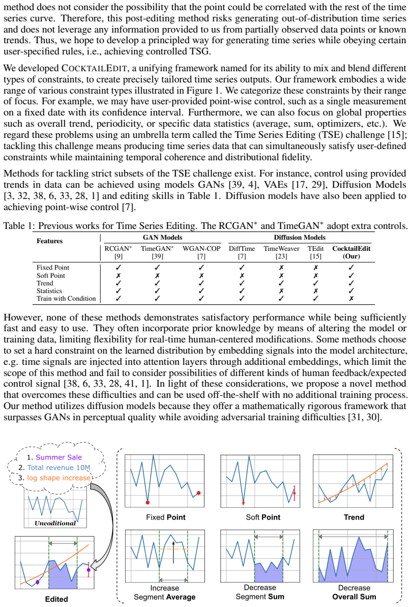
The central discovery is that multi-grained time series editing can be reduced to two sampling-time mechanisms that do not require touching the model. First, point-wise constraints are enforced by a confidence-weighted float mask: at every denoising step the observed anchor values are propagated through the forward noising process to the current noise level and combined with the denoised trajectory via $x_t \leftarrow \omega_t m \odot x_t^{\mathrm{ob}} + (1-\omega_t m)\odot x_t^{\mathrm{ta}}$, where $m$ is the per-point confidence and $\omega_t=\exp(-\gamma t/T)$ strengthens control as $t\to 0$. Second, segment-level statistics are enforced by a classifier-style penalty such as $\mathcal{L}_{\mathrm{sum}}=(\sum_{i=s_j}^{e_j}x_{t,i}-S_{\mathrm{target}})^2$ added to the score gradient. Interleaving the two during sampling yields edited series that respect anchors exactly at full confidence and move segment sums monotonically with the requested target, while the paper's own distribution metrics show the edits come at the cost of moving the samples away from the original data distribution.
Load-bearing premise
The method's load-bearing premise is that mixing forward-noised observed anchor values into the denoising trajectory at every step, weighted by a float mask, produces samples from the true conditional distribution given those anchors; if that blending is not exact conditional sampling, the edited series drift out of distribution, which the paper's own distribution-shift scores suggest is happening.
Editorial extensions
If this is right
- Any conditionally trained diffusion model for time series can be edited at inference time: point anchors and segment statistics are enforced purely by masks and gradients, so no model weights change.
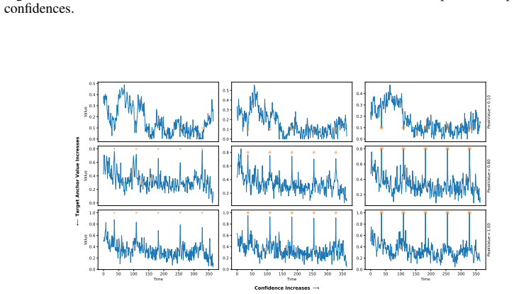
- Full confidence ($m=1$) on an anchor forces the generated value at that index to match the anchor exactly (MAD converging to 0.0 in the reported tables), while intermediate confidence gives a controllable trade-off between fidelity to the anchor and fidelity to the learned temporal dynamics.
- Target segment sums respond monotonically to the requested value: on the Revenue dataset, targeting 150.0 raises the generated sequence sum from about 76.6 to 117.9, and targeting -100.0 lowers it to about 52.7 (Table 4, Diffusion-TS backbone).
- The same sampling-time mechanism covers trend control (by interpolating a reference trend into dense point anchors) and combined multi-granularity control, with near-zero added runtime per sample (Table 6).
- Distribution preservation and control precision trade off: discriminative scores, Context-FID, and correlational scores rise after control is applied, so stronger control moves the output away from the original data distribution.
Reading between the lines
- The paper does not test it, but replacing the sum penalty in Eq. 14 with any differentiable aggregate—volatility, peak, correlation, or a weighted average—should work the same way, so the claimed statistics control is plausibly a general mechanism rather than a sum-only trick.
- If the mask-blending equivalence from Appendix A.2 were exactly true, intermediate-confidence edits should coincide with samples from a model natively trained to condition on the same anchors; comparing CocktailEdit against such a conditional model would either confirm the theory or expose the distribution drift the reported FID/discriminative scores hint at.
- The time-dependent weight $\omega_t$ and dynamic mask adjustment are heuristics; making the schedule part of a proper stochastic-differential-equation guidance term could connect this to exact conditional sampling and might remove the control–fidelity trade-off.
- The interactive editor described in the paper is a screen demo; the per-sample cost of 0.06–9.6 ms suggests the same machinery could drive live, drag-to-edit tools for forecasting and what-if analysis, not just offline generation.
Editorial analysis
A structured set of objections, weighed in public.
Referee Report
Summary. The paper proposes CocktailEdit, an inference-time framework for editing time series generated by pretrained conditional diffusion models. Point-level constraints are enforced by blending forward-noised observed values with denoised target values via a confidence mask and a time-dependent weight (Eqs. 8 and 10), while segment-level statistics such as sums are controlled by adding an L2 penalty on the segment sum during sampling (Eqs. 14 and 15). The method is evaluated on ETTh, fMRI, Revenue, and Sines with CSDI and Diffusion-TS backbones. The experiments show that higher confidence values reduce the mean absolute difference at anchor points and that sum control shifts the achieved sums in the requested direction, at the cost of substantially increased distribution-divergence metrics. The paper claims that this is a principled, training-free way to enforce multi-grained constraints while maintaining temporal coherence and distributional fidelity.
Significance. If the central claim were established, the framework would be practically useful: it offers a plug-and-play way to impose anchors and segment statistics on any conditionally trained diffusion model. The paper has real strengths: it ships code and a demo, evaluates on multiple backbones and datasets, reports time efficiency, and openly acknowledges distribution drift in the conclusion. However, the main theoretical guarantee is not proven, and the empirical distribution-fidelity results contradict the abstract's claim of maintaining distributional fidelity. As a heuristic editing tool, the point-control component appears to work as expected, but the paper currently frames it as a principled conditional-sampling procedure, which is the load-bearing weakness.
major comments (4)
- [Appendix A.2, Eq. (10)] The proof in Appendix A.2 does not establish that the float-mask update in Eq. (10) samples from p(x_ta | x_ob). Step III asserts that blending with a float mask keeps the observed indices consistent, but for m < 1 and omega_t < 1 the observed coordinate becomes a convex combination of the forward-noised observation and the generated coordinate, so it is not the forward-sampled value. Step IV simply restates the desired limit without argument, and Eq. (7) conditions the reverse transition on x_ob^t in a nonstandard way without deriving the score of the conditional process. Because the paper motivates confidence masking as a principled conditional-sampling mechanism, this gap is load-bearing; as written, the update is a heuristic blend rather than a derivation.
- [Section 5.3, Tables 9 and 11] The distribution-fidelity claim in the abstract and introduction is contradicted by the paper's own metrics. With the Diffusion-TS backbone, point control raises the ETTh Context-FID from 0.108 +/- 0.007 to 7.797 +/- 0.644 at confidence 0.01 and the discriminative score from 0.034 +/- 0.026 to 0.437 +/- 0.004; large degradations also appear for statistics control. The conclusion explicitly admits that 'obvious distribution drift still exists.' These results should be reconciled with the claim that the method maintains distributional fidelity, either by removing that claim or by providing evidence that the trade-off is acceptable in a well-defined sense.
- [Sections 3.5 and 5.2, Eqs. (13)-(15), Table 4] The statistics-control mechanism is a direct L2 penalty on the segment sum, not classifier guidance as claimed. The classifier p_phi in Eq. (13) is never defined or trained, and Eq. (14) is an explicit mean-squared-error term on the raw sum. Moreover, the control does not reach its targets in several settings: for Sines, the target 150 yields an achieved sum of 21.031 (nearly the same as the target 20 result of 20.146), and for Revenue the target -100 yields 52.675 versus an unconditional 76.619; the CSDI results in Appendix D.1.2 are even less responsive. Please rename the mechanism, define any auxiliary model, and report relative target error or success rates rather than only directional movement.
- [Section 5.1, Eq. (10)] The monotonic decrease of MAD with confidence, and the exact zero at confidence 1.0, follow by construction from Eq. (10): setting m = 1 forces x_t to equal x_ob^t, and the forward noising process tends to x_ob^0 as t approaches 0. The empirical MAD curve is therefore a sanity check of the mask implementation, not evidence for the unproven conditional-sampling claim in Appendix A.2. The text should not present this behavior as a theoretical validation of conditional correctness.
minor comments (6)
- [Abstract] The sentence 'Time Series Editing (TSE) - making precise modifications while preserving temporal coherence - current methods struggle...' is not grammatical, and 'integrating seamlessly, with any conditionally trained' contains a stray comma. Please revise for clarity.
- [Section 3.2, Eq. (7)] Equation (7) appears to condition p_theta on its own argument, x_{t+1}^{ta} | x_{t+1}^{ta}, which is likely a typo in the indices. Please correct the notation.
- [Algorithm 1, line 13] The point-wise mask is applied to x_t, but the preceding steps produce x_{t-1}; the index convention is inconsistent with Eq. (10). Please clarify the update order and define m_ob.
- [Table 3 and Table 6] The ETTh panel in Table 3 lists target value 0.8 twice and omits 0.5, and Table 6 uses the name 'Energy' while the rest of the paper uses 'ETTh'. These inconsistencies should be fixed.
- [Appendix B] Appendix B states that 'we will include the various sequence length results, such L in {96, 192, 384} in the camera-ready version.' This is inappropriate for a submitted manuscript and should be removed or replaced with the actual results.
- [Figures 33-36 and Table 4] The achieved sums reported in the figure captions appear inconsistent with Table 4 (for example, ETTh target 20 gives 8.502 in Table 4 but the corresponding caption reports 'Sum: 10.0'). Please reconcile the numbers or clarify whether different settings were used.
Circularity Check
Float-mask blending is not derived from the conditional score; the A.2 proof restates the conclusion, MAD at confidence=1 and its monotonic decrease are forced by Eq. 10, and sum-control 'results' are the optimized loss itself.
-
self definitional
[Section 3.2, Eq. 10; Section 5.1, Table 3]
"When wi = 1, we rely entirely on the observed data; when wi = 0, the model-generated sample is used. ... xt ←ω tm⊙x ob t + (1−ω tm)⊙x ta t . ... This convergence at confidence = 1.0 validates our theoretical guarantee that maximum confidence forces the point to be a fixed point."
With wi = 1, mask m = 1 and the update Eq. 10 gives xt = ωt x_ob^t + (1−ωt) x_ta^t. Since ωt = exp(−γ t/num_timesteps) tends to 1 as t→0, the final value is exactly the forward-noised observed value x_ob^0, which converges to the anchor. Therefore MAD = 0 at confidence = 1 is a direct algebraic consequence of the mask definition, not an empirical validation of a prediction. The same construction forces the reported 'convergence'.
-
self definitional
[Section 5.1, Figure 2]
"The monotonic and linear decrease of MAD with increasing confidence is visualized in Figure 2."
Eq. 10 defines the controlled iterate as a convex combination of x_ob^t (the forward-noised anchor) and x_ta^t (the generated sample). Increasing the confidence m linearly increases the weight on the anchor branch, so the final value moves monotonically toward the anchor by construction. Reporting this as an experimental finding about 'higher confidence values lead to more precise point control' is reporting the definition of the blending rule, not an independent result.
2 more flagged steps
-
other
[Appendix A.2, Step IV]
"Consider pt(xt ta |x t ob). By the score-based argument (the forward-reverse chain forming a time-indexed Markov process), the mixture of denoising steps and partial resets of observed entries yields lim t→0 pt(xt ta |x t ob) =p(x ta |x ob), where the convergence follows from the fact that each reverse diffusion step corrects the noise injected in the forward pass, conditioned on the known x t ob."
This is the theorem to be proved, restated without a derivation. Step III asserts that for a float mask the observed indices 'remain consistent', but for m < 1 and ωt < 1 the coordinate is a convex combination of x_ob^t and x_ta^t, so it is not the forward-sampled observed marginal. Step IV then simply asserts the desired conditional limit, citing the generic score-based argument rather than showing that the float-mask reset defines the reverse transition of the conditional process. The proof therefore assumes the conclusion.
-
fitted input called prediction
[Section 3.5, Eq. 14; Section 4.3; Section 5.2, Table 4]
"Lsum[sj :ej ] = ( sum_{i=sj}^{ej} x_{t,i} −S target[sj :ej ] )^2 ... the control target function is the sum of series, we directly observe the actual sum value change to validate the controllability."
The 'Statistic Control Result' reports the very quantity that the algorithm explicitly minimizes: the squared difference between the generated segment sum and the target sum. Gradient descent on this loss will move the sum toward the target by construction, so Table 4 is a check that the optimizer reduces its own objective, not an independent prediction or derivation. The claimed controllability is thus equivalent to the definition of the penalty term.
full rationale
The central derivation of CocktailEdit is not self-contained: the formal proof in Appendix A.2 claims that float-mask blending samples from the true conditional distribution, but Step IV restates the desired limit and Step III's consistency claim is false for fractional masks. Separately, the point-wise 'validation' is definitional: confidence = 1 forces MAD = 0 through Eq. 10, and the monotone MAD decrease is the algebraic behavior of a convex combination with increasing anchor weight. The sum-control experiments similarly report the value of the loss being minimized, so they reduce to the optimization objective. No load-bearing self-citation chain is present: the cited score-based convergence is external, though it is misapplied to the blended process. The paper itself concedes 'obvious distribution drift still exists', and its own Context-FID and discriminative tables show large shifts, which is consistent with the failure of the A.2 claim. The framework may still be a useful heuristic editor, but its claimed conditional-sampling guarantee and several reported 'results' are circular by construction, giving a partial-circularity score of 6.
Assumptions & free parameters
free parameters (4)
- gamma (time-dependent weight exponent) =
5.0 (from Appendix A.3)
- eta (gradient scale) =
not reported
- beta_sum (sum-control weights) =
range {1,10,50,100} tested
- lambda_1, lambda_2, lambda_3 (mask reweighting) =
not reported
assumptions (4)
- ad hoc to paper A float-mask blend of forward-noised observed values and reverse-denoised target values at every step yields samples from p(x_ta | x_ob).
- ad hoc to paper A direct L2 penalty on segment sums is equivalent to classifier guidance for conditioning.
- standard math DDPM reverse process approximates the true score and can be conditioned via guidance.
- domain assumption The pretrained diffusion models (CSDI, Diffusion-TS) are sufficiently well-trained for the task.
Cite this review
Pith. "Pith review of How to Unlock Time Series Editing? Diffusion-Driven Approach with Multi-Grained Control." pith.science (2026). https://pith.science/paper/J5XG4OSU
@misc{pith2026250605276,
  author       = {Pith},
  title        = {Pith review of: How to Unlock Time Series Editing? Diffusion-Driven Approach with Multi-Grained Control},
  year         = {2026},
  howpublished = {\url{https://pith.science/paper/J5XG4OSU}},
  note         = {Machine review of arXiv:2506.05276}
}
read the original abstract
Recent advances in time series generation have shown promise, yet controlling properties in generated sequences remains challenging. Time Series Editing (TSE) - making precise modifications while preserving temporal coherence - consider both point-level constraints and segment-level controls that current methods struggle to provide. We introduce the CocktailEdit framework to enable simultaneous, flexible control across different types of constraints. This framework combines two key mechanisms: a confidence-weighted anchor control for point-wise constraints and a classifier-based control for managing statistical properties such as sums and averages over segments. Our methods achieve precise local control during the denoising inference stage while maintaining temporal coherence and integrating seamlessly, with any conditionally trained diffusion-based time series models. Extensive experiments across diverse datasets and models demonstrate its effectiveness. Our work bridges the gap between pure generative modeling and real-world time series editing needs, offering a flexible solution for human-in-the-loop time series generation and editing. The code and demo are provided for validation.
Figures


Figures from the paper (64 more)




Reference graph
Works this paper leans on
-
[1]
Fernandez, Fatemeh Afghah, and John J
Edmonmd Adib, Amanda S. Fernandez, Fatemeh Afghah, and John J. Prevost. Synthetic ecg signal generation using probabilistic diffusion models.IEEE Access, 11:75818–75828, 2024
work page 2024
-
[2]
Juan Miguel Lopez Alcaraz and Nils Strodthoff. Diffusion-based time series imputation and forecasting with structured state space models.Version published by Transactions on Machine Learning Research in 2022 (TMLR ISSN 2835-8856) https://openreview.net/forum?id=hHiIbk7ApW, August 2022
work page 2022
-
[3]
Yihao Ang, Qiang Huang, Yifan Bao, Anthony K. H. Tung, and Zhiyong Huang. Tsgbench: Time series generation benchmark. September 2023
work page 2023
-
[4]
Gaby Baasch, Guillaume Rousseau, and Ralph Evins. A conditional generative adversarial network for energy use in multiple buildings using scarce data.Energy and AI, 5:100087, 2021
work page 2021
-
[5]
Yifan Bao, Yihao Ang, Qiang Huang, Anthony K. H. Tung, and Zhiyong Huang. Towards controllable time series generation. March 2024
work page 2024
-
[6]
Timedit: General-purpose diffusion transformers for time series foundation model
Defu Cao, Wen Ye, Yizhou Zhang, and Yan Liu. Timedit: General-purpose diffusion transformers for time series foundation model. September 2024
work page 2024
-
[7]
On the constrained time-series generation problem
Andrea Coletta, Sriram Gopalakrishnan, Daniel Borrajo, and Svitlana Vyetrenko. On the constrained time-series generation problem. In A. Oh, T. Naumann, A. Globerson, K. Saenko, M. Hardt, and S. Levine, editors,Advances in Neural Information Processing Systems, volume 36, pages 61048–61059. Curran Associates, Inc., 2023
work page 2023
-
[8]
Timevae: A variational auto-encoder for multivariate time series generation
Abhyuday Desai, Cynthia Freeman, Zuhui Wang, and Ian Beaver. Timevae: A variational auto-encoder for multivariate time series generation. November 2021. 9
work page 2021
Show all 42 references
-
[9]
Hyland, and Gunnar Rätsch
Cristóbal Esteban, Stephanie L. Hyland, and Gunnar Rätsch. Real-valued (medical) time series generation with recurrent conditional gans. June 2017
2017
-
[10]
Latent diffusion transformer for probabilistic time series forecasting.Proceedings of the AAAI Conference on Artificial Intelligence, 38(11):11979–11987, Mar
Shibo Feng, Chunyan Miao, Zhong Zhang, and Peilin Zhao. Latent diffusion transformer for probabilistic time series forecasting.Proceedings of the AAAI Conference on Artificial Intelligence, 38(11):11979–11987, Mar. 2024
2024
-
[11]
Nips 2016 tutorial: Generative adversarial networks.arXiv preprint arXiv:1701.00160, 2016
Ian Goodfellow. Nips 2016 tutorial: Generative adversarial networks.arXiv preprint arXiv:1701.00160, 2016
2016 arXiv
-
[12]
Generative modeling for time series via schrödinger bridge
Mohamed Hamdouche, Pierre Henry-Labordere, and Huyên Pham. Generative modeling for time series via schrödinger bridge. April 2023
2023
-
[13]
Denoising diffusion probabilistic models
Jonathan Ho, Ajay Jain, and Pieter Abbeel. Denoising diffusion probabilistic models. June 2020
2020
-
[14]
Li, Sheng Wang, and Tianlong Chen
Yang Hu, Xiao Wang, Lirong Wu, Huatian Zhang, Stan Z. Li, Sheng Wang, and Tianlong Chen. Fm-ts: Flow matching for time series generation. November 2024
2024
-
[15]
Towards editing time series
Baoyu Jing, Shuqi Gu, Tianyu Chen, Zhiyu Yang, Dongsheng Li, Jingrui He, and Kan Ren. Towards editing time series. InThe Thirty-eighth Annual Conference on Neural Information Processing Systems, 2024
2024
-
[16]
Diffwave: A versatile diffusion model for audio synthesis.arXiv preprint arXiv:2009.09761, 2020
Zhifeng Kong, Wei Ping, Jiaji Huang, Kexin Zhao, and Bryan Catanzaro. Diffwave: A versatile diffusion model for audio synthesis.arXiv preprint arXiv:2009.09761, 2020
2009 arXiv
-
[17]
Vector quantized time series generation with a bidirectional prior model
Daesoo Lee, Sara Malacarne, and Erlend Aune. Vector quantized time series generation with a bidirectional prior model. March 2023
2023
-
[18]
Generative time series forecasting with diffusion, denoise, and disentanglement
Yan Li, Xinjiang Lu, Yaqing Wang, and Dejing Dou. Generative time series forecasting with diffusion, denoise, and disentanglement. In S. Koyejo, S. Mohamed, A. Agarwal, D. Belgrave, K. Cho, and A. Oh, editors,Advances in Neural Information Processing Systems, volume 35, pages ...
2022
-
[19]
Retrieval-augmented diffusion models for time series forecasting
Jingwei Liu, Ling Yang, Hongyan Li, and Shenda Hong. Retrieval-augmented diffusion models for time series forecasting. October 2024
2024
-
[20]
Deep time series forecasting models: A comprehensive survey.Mathematics, 12(10), 2024
Xinhe Liu and Wenmin Wang. Deep time series forecasting models: A comprehensive survey.Mathematics, 12(10), 2024
2024
-
[21]
Caspar Meijer and Lydia Y . Chen. The rise of diffusion models in time-series forecasting. January 2024
2024
-
[22]
Generative semi- supervised learning for multivariate time series imputation
Xiaoye Miao, Yangyang Wu, Jun Wang, Yunjun Gao, Xudong Mao, and Jianwei Yin. Generative semi- supervised learning for multivariate time series imputation. InProceedings of the AAAI conference on artificial intelligence, volume 35, pages 8983–8991, 2021
2021
-
[23]
Time weaver: A conditional time series generation model
Sai Shankar Narasimhan, Shubhankar Agarwal, Oguzhan Akcin, Sujay Sanghavi, and Sandeep Chinchali. Time weaver: A conditional time series generation model. March 2024
2024
-
[24]
Temporal latent auto-encoder: A method for probabilistic multivariate time series forecasting
Nam Nguyen and Brian Quanz. Temporal latent auto-encoder: A method for probabilistic multivariate time series forecasting. InProceedings of the AAAI conference on artificial intelligence, volume 35, pages 9117–9125, 2021
2021
-
[25]
Leveraging priors via diffusion bridge for time series generation
Jinseong Park, Seungyun Lee, Woojin Jeong, Yujin Choi, and Jaewook Lee. Leveraging priors via diffusion bridge for time series generation. August 2024
2024
-
[26]
Variational autoencoder
Lucas Pinheiro Cinelli, Matheus Araújo Marins, Eduardo Antúnio Barros da Silva, and Sérgio Lima Netto. Variational autoencoder. InVariational Methods for Machine Learning with Applications to Deep Networks, pages 111–149. Springer, 2021
2021
-
[27]
Autoregressive denoising diffusion models for multivariate probabilistic time series forecasting
Kashif Rasul, Calvin Seward, Ingmar Schuster, and Roland V ollgraf. Autoregressive denoising diffusion models for multivariate probabilistic time series forecasting. In Marina Meila and Tong Zhang, editors, Proceedings of the 38th International Conference on Machine Learning, ...
2021
-
[28]
Diff-mts: Temporal-augmented conditional diffusion-based aigc for industrial time series toward the large model era.IEEE Transactions on Cybernetics, 54(12):7187–7197, 2024
Lei Ren, Haiteng Wang, and Yuanjun Laili. Diff-mts: Temporal-augmented conditional diffusion-based aigc for industrial time series toward the large model era.IEEE Transactions on Cybernetics, 54(12):7187–7197, 2024
2024
-
[29]
A survey of transformer enabled time series synthesis
Alexander Sommers, Logan Cummins, Sudip Mittal, Shahram Rahimi, Maria Seale, Joseph Jaboure, and Thomas Arnold. A survey of transformer enabled time series synthesis. June 2024. 10
2024
-
[30]
Denoising diffusion implicit models
Jiaming Song, Chenlin Meng, and Stefano Ermon. Denoising diffusion implicit models. October 2020
2020
-
[31]
Kingma, Abhishek Kumar, Stefano Ermon, and Ben Poole
Yang Song, Jascha Sohl-Dickstein, Diederik P. Kingma, Abhishek Kumar, Stefano Ermon, and Ben Poole. Score-based generative modeling through stochastic differential equations. November 2020
2020
-
[32]
Csdi: Conditional score-based diffusion models for probabilistic time series imputation
Yusuke Tashiro, Jiaming Song, Yang Song, and Stefano Ermon. Csdi: Conditional score-based diffusion models for probabilistic time series imputation. In M. Ranzato, A. Beygelzimer, Y . Dauphin, P.S. Liang, and J. Wortman Vaughan, editors,Advances in Neural Information Processin...
2021
-
[33]
Muhang Tian, Bernie Chen, Allan Guo, Shiyi Jiang, and Anru R Zhang. Reliable generation of privacy- preserving synthetic electronic health record time series via diffusion models.Journal of the American Medical Informatics Association, 31(11):2529–2539, 09 2024
2024
-
[34]
Torres, Dalil Hadjout, Abderrazak Sebaa, Francisco Martínez-Álvarez, and Alicia Troncoso
José F. Torres, Dalil Hadjout, Abderrazak Sebaa, Francisco Martínez-Álvarez, and Alicia Troncoso. Deep learning for time series forecasting: A survey.Big Data, 9(1):3–21, February 2021
2021
-
[35]
Deep time series models: A comprehensive survey and benchmark
Yuxuan Wang, Haixu Wu, Jiaxiang Dong, Yong Liu, Mingsheng Long, and Jianmin Wang. Deep time series models: A comprehensive survey and benchmark. July 2024
2024
-
[36]
Diffstg: Probabilistic spatio-temporal graph forecasting with denoising diffusion models
Haomin Wen, Youfang Lin, Yutong Xia, Huaiyu Wan, Qingsong Wen, Roger Zimmermann, and Yuxuan Liang. Diffstg: Probabilistic spatio-temporal graph forecasting with denoising diffusion models. In Proceedings of the 31st ACM International Conference on Advances in Geographic Inform...
2023
-
[37]
Quant gans: deep generation of financial time series.Quantitative Finance, 20(9):1419–1440, 2020
Magnus Wiese, Robert Knobloch, Ralf Korn, and Peter Kretschmer. Quant gans: deep generation of financial time series.Quantitative Finance, 20(9):1419–1440, 2020
2020
-
[38]
Diffusion-based time series data imputation for cloud failure prediction at microsoft 365
Fangkai Yang, Wenjie Yin, Lu Wang, Tianci Li, Pu Zhao, Bo Liu, Paul Wang, Bo Qiao, Yudong Liu, Mårten Björkman, Saravan Rajmohan, Qingwei Lin, and Dongmei Zhang. Diffusion-based time series data imputation for cloud failure prediction at microsoft 365. InProceedings of the 31s...
2023
-
[39]
Time-series generative adversarial networks
Jinsung Yoon, Daniel Jarrett, and Mihaela van der Schaar. Time-series generative adversarial networks. In H. Wallach, H. Larochelle, A. Beygelzimer, F. d'Alché-Buc, E. Fox, and R. Garnett, editors,Advances in Neural Information Processing Systems, volume 32. Curran Associates,...
2019
-
[40]
Diffusion-ts: Interpretable diffusion for general time series generation
Xinyu Yuan and Yan Qiao. Diffusion-ts: Interpretable diffusion for general time series generation. March 2024
2024
-
[41]
Zhang, S
S. Zhang, S. Wang, H. Miao, H. Chen, C. Fan, and J. Zhang. Score-cdm: Score-weighted convolutional diffusion model for multivariate time series imputation. May 2024
2024
-
[42]
Denoising diffusion bridge models
Linqi Zhou, Aaron Lou, Samar Khanna, and Stefano Ermon. Denoising diffusion bridge models. September 2023. 11 A Methodology Additional Details A.1 Summary of Variants Table 7: Summary of variables and their Meanings Symbol Meaning NNumber of time series xi ∈R L×D i-th time ser...
2023
Reviewed August 7, 2026 · model on record in the stance chip above.
Discussion (0). Sign in to comment.