From Landau Equation and Large Deviations to Efficient Simulations of Dynamical Fluctuations
Pith reviewed 2026-06-26 12:43 UTC · model grok-4.3
The pith
A set of Langevin equations recovers the mean Landau dynamics while capturing fluctuations among realizations in long-range interacting systems.
A machine-rendered reading of the paper's core claim, the machinery that carries it, and where it could break.
Core claim
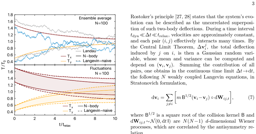
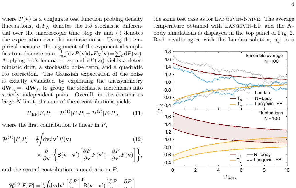
Building upon Large Deviation Theory, we present a physically-consistent system of Langevin equations that simultaneously recovers the mean Landau dynamics and accurately captures the corresponding fluctuations among different realizations. We show in particular how these Langevin equations can be derived from Rostoker's principle in the limit of weak two-body deflections. We extensively validate these equations against tailored direct N-body simulations, showing an exquisite level of agreement.
What carries the argument
The system of Langevin equations obtained from Rostoker's principle in the weak-deflection limit, which augments the Landau collision operator with consistent noise terms to generate fluctuation statistics.
Load-bearing premise
The noise term is justified only when Rostoker's principle governs the fluctuation statistics in the limit of weak two-body deflections.
What would settle it
Direct N-body runs in a regime of strong two-body deflections where the observed fluctuation variance deviates systematically from the variance predicted by the derived noise term.
Figures
read the original abstract
The (deterministic) Landau equation captures the mean long-term evolution of dynamically hot long-range interacting finite-$N$ systems. Though successful, this kinetic equation fundamentally ignores dynamical fluctuations. Building upon Large Deviation Theory, we present a physically-consistent system of Langevin equations that simultaneously recovers the mean Landau dynamics and accurately captures the corresponding fluctuations among different realizations. We show in particular how these Langevin equations can be derived from Rostoker's principle in the limit of weak two-body deflections. We extensively validate these equations against tailored direct $N$-body simulations, showing an exquisite level of agreement.
Editorial analysis
A structured set of objections, weighed in public.
Referee Report
Summary. The manuscript derives a system of Langevin equations from large deviation theory that recovers the deterministic Landau equation for the mean evolution of finite-N long-range interacting systems while also describing realization-to-realization fluctuations. The derivation invokes Rostoker's principle in the weak two-body deflection limit to obtain the noise term, and the equations are validated against direct N-body simulations with claimed excellent agreement.
Significance. If the central derivation holds, the work provides an efficient stochastic framework for simulating dynamical fluctuations in systems governed by the Landau equation (e.g., plasmas, gravitational clusters) without requiring full N-body integration for every realization. The explicit use of large deviation theory to link mean kinetics and fluctuations is a conceptual strength, as is the parameter-free character asserted in the abstract.
major comments (2)
- [Derivation via Rostoker's principle] Derivation of the multiplicative noise correlator (section on Rostoker's principle application): Rostoker's principle is standard for the deterministic Landau collision integral, but the step extending it to the large-deviation rate function or the corresponding noise term for fluctuation statistics is not automatic. The manuscript must explicitly demonstrate that the weak-deflection limit yields the correct second-moment correlator without additional assumptions; otherwise the claim that the Langevin system simultaneously recovers both mean dynamics and correct fluctuations is not justified.
- [Validation section] Validation against N-body simulations (results section): The abstract asserts 'exquisite level of agreement,' but without reported error bars, number of independent realizations, specific observables compared (e.g., variance of energy or density fluctuations), or data-selection criteria, it is impossible to assess whether the fluctuation spectrum is accurately reproduced or whether discrepancies are hidden by averaging.
minor comments (2)
- Notation for the Langevin noise term should be clarified to distinguish it from the standard Landau operator; a table comparing the deterministic Landau equation, the large-deviation rate function, and the final stochastic equations would improve readability.
- The abstract mentions 'tailored direct N-body simulations'; the methods section should specify the integration scheme, softening length, and how initial conditions were sampled to ensure reproducibility.
Simulated Author's Rebuttal
We thank the referee for the constructive report and the positive assessment of the work's significance. We address the two major comments below, indicating the revisions that will be incorporated.
read point-by-point responses
-
Referee: Derivation of the multiplicative noise correlator (section on Rostoker's principle application): Rostoker's principle is standard for the deterministic Landau collision integral, but the step extending it to the large-deviation rate function or the corresponding noise term for fluctuation statistics is not automatic. The manuscript must explicitly demonstrate that the weak-deflection limit yields the correct second-moment correlator without additional assumptions; otherwise the claim that the Langevin system simultaneously recovers both mean dynamics and correct fluctuations is not justified.
Authors: We agree that the connection between Rostoker's principle and the noise correlator requires explicit verification. The manuscript derives the Langevin system by substituting the large-deviation rate function into Rostoker's weak-deflection framework and obtains the multiplicative noise whose second moment is fixed by the same two-body scattering kernel that appears in the Landau integral. To make this step fully transparent, the revised version will include a dedicated paragraph that computes the second-moment correlator directly from the deflection-angle expansion, confirming that no auxiliary assumptions are introduced beyond the standard weak-scattering limit already used for the mean dynamics. revision: yes
-
Referee: Validation against N-body simulations (results section): The abstract asserts 'exquisite level of agreement,' but without reported error bars, number of independent realizations, specific observables compared (e.g., variance of energy or density fluctuations), or data-selection criteria, it is impossible to assess whether the fluctuation spectrum is accurately reproduced or whether discrepancies are hidden by averaging.
Authors: The referee correctly identifies that quantitative details supporting the agreement claim are missing from the current presentation. In the revised manuscript we will augment the validation section with: (i) error bars obtained from the standard deviation across independent runs, (ii) the number of realizations performed (typically 50–100 depending on N), (iii) explicit comparison of both the mean evolution and the fluctuation observables (energy variance, density fluctuation spectrum, and two-point correlation functions), and (iv) a clear statement of the time-window and ensemble-selection criteria used for the reported curves. revision: yes
Circularity Check
No circularity: derivation from external Rostoker + LDT principles
full rationale
The paper states it derives the Langevin system from Rostoker's principle (standard collision operator) in the weak-deflection limit plus large-deviation theory. These are external inputs, not defined inside the paper. No equation reduces a fluctuation correlator to a fitted parameter by construction, and no load-bearing self-citation chain appears. Validation against independent N-body runs supplies an external benchmark. The derivation chain therefore remains self-contained against external standards.
Axiom & Free-Parameter Ledger
axioms (1)
- domain assumption Rostoker's principle applies to the fluctuation statistics in the weak-deflection limit
Reference graph
Works this paper leans on
-
[1]
Campa, T
A. Campa, T. Dauxois, D. Fanelli, and S. Ruffo,Physics of long-range interacting systems(Oxford Univ. Press, 2014)
2014
-
[2]
D. R. Nicholson,Introduction to Plasma Theory (Krieger, 1992)
1992
-
[3]
Binney and S
J. Binney and S. Tremaine,Galactic Dynamics: Second Edition(Princeton Univ. Press, 2008)
2008
-
[4]
D. C. Heggie and P. Hut,The gravitational million-body problem(Cambridge Univ. Press, 2003)
2003
-
[5]
Bouchet and A
F. Bouchet and A. Venaille, Phys. Rep.515, 227 (2012)
2012
-
[6]
Dauxois, S
T. Dauxois, S. Ruffo, E. Arimondo, and M. Wilkens, in Dynamics and Thermodynamics of Systems with Long- Range Interactions(Springer, 2002), vol. 602, pp. 1–19
2002
-
[7]
Y. L. Klimontovich,The Statistical Theory of Non- Equilibrium Processes in a Plasma(Elsevier, 1967)
1967
-
[8]
Balescu,Statistical Dynamics: Matter out of Equilib- rium(Imperial Coll., London, 1997)
R. Balescu,Statistical Dynamics: Matter out of Equilib- rium(Imperial Coll., London, 1997)
1997
-
[9]
E. M. Lifshitz and L. P. Pitaevskii,Physical kinetics (Pergamon Press, 1981)
1981
-
[10]
Hamilton and J.-B
C. Hamilton and J.-B. Fouvry, Phys. Plasmas31, 120901 (2024)
2024
-
[11]
L. D. Landau, Phys. Z. Sowj. Union10, 154 (1936)
1936
-
[12]
Lynden-Bell and R
D. Lynden-Bell and R. Wood, MNRAS138, 495 (1968)
1968
-
[13]
Roule, J.-B
M. Roule, J.-B. Fouvry, C. Pichon, and P.-H. Chavanis, A&A699, A140 (2025)
2025
- [14]
-
[15]
Touchette, Phys
H. Touchette, Phys. Rep.478, 1 (2009)
2009
-
[16]
Feliachi and F
O. Feliachi and F. Bouchet, J. Stat. Phys.183, 42 (2021)
2021
-
[17]
Feliachi and F
O. Feliachi and F. Bouchet, J. Stat. Phys.186, 22 (2022)
2022
-
[18]
Feliachi and J.-B
O. Feliachi and J.-B. Fouvry, Phys. Rev. E110, 024108 (2024)
2024
-
[19]
Fontbona, H
J. Fontbona, H. Gu´ erin, and S. M´ el´ eard, Probab. Theory Relat. Fields143, 329 (2009)
2009
-
[20]
Y. Fu, J. R. Angus, H. Qin, and V. I. Geyko, Phys. Rev. E111, 025211 (2025)
2025
-
[21]
See Supplemental Material
-
[22]
Chavanis, A&A556, A93 (2013)
P.-H. Chavanis, A&A556, A93 (2013)
2013
-
[23]
Bouchet, T
F. Bouchet, T. Grafke, T. Tangarife, and E. Vanden- Eijnden, J. Stat. Phys.162, 793 (2016)
2016
-
[24]
Bertini, A
L. Bertini, A. De Sole, D. Gabrielli, G. Jona-Lasinio, and C. Landim, Rev. Mod. Phys.87, 593 (2015)
2015
-
[25]
Risken,The Fokker-Planck equation(Springer, 1989)
H. Risken,The Fokker-Planck equation(Springer, 1989). 6
1989
-
[26]
Heyvaerts, J.-B
J. Heyvaerts, J.-B. Fouvry, P.-H. Chavanis, and C. Pi- chon, MNRAS469, 4193 (2017)
2017
-
[27]
Rostoker, Phys
N. Rostoker, Phys. Fluids7, 479 (1964)
1964
-
[28]
Rostoker, Phys
N. Rostoker, Phys. Fluids7, 491 (1964)
1964
-
[29]
K. Du, L. Li, Y. Xie, and Y. Yu, J. Comp. Phys.543, 114387 (2025)
2025
-
[30]
Bouchet, C
F. Bouchet, C. Nardini, and T. Tangarife, J. Stat. Phys. 153, 572 (2013)
2013
-
[31]
D. S. Dean, J. Phys. A29, L613 (1996)
1996
-
[32]
Kawasaki, J
K. Kawasaki, J. Stat. Phys.93, 527 (1998)
1998
-
[33]
Cornalba and J
F. Cornalba and J. Fischer, Arch. Ration. Mech. Anal. 247, 76 (2023)
2023
-
[34]
Balescu, Phys
R. Balescu, Phys. Fluids3, 52 (1960)
1960
-
[35]
Lenard, Ann
A. Lenard, Ann. Phys. (N.-Y.)10, 390 (1960). [36]https://github.com/anwar-elrhirhayi/Langevin_ Landau
1960
-
[36]
Hamilton, MNRAS501, 3371 (2021)
C. Hamilton, MNRAS501, 3371 (2021)
2021
-
[37]
Bhattacharya and E
R. Bhattacharya and E. C. Waymire,The Functional Central Limit Theorem (FCLT)(Springer, 2021)
2021
-
[38]
Hairer, C
E. Hairer, C. Lubich, and G. Wanner,Geometric numer- ical integration: Second Edition(Springer, 2006)
2006
-
[39]
Yoshida, Phys
H. Yoshida, Phys. Lett. A150, 262 (1990)
1990
-
[40]
Kloeden and E
P. Kloeden and E. Platen,Numerical Solution of Stochas- tic Differential Equations(Springer, 2011)
2011
-
[41]
Hong and L
J. Hong and L. Sun,Stochastic Structure-Preserving Nu- merical Methods(Springer, 2022)
2022
-
[42]
Zhang, Y
X. Zhang, Y. Fu, and H. Qin, Phys. Rev. E102(2020)
2020
-
[43]
Bouchet, J
F. Bouchet, J. Stat. Phys.181, 515 (2020). 7 End Matter ROSTOKER APPROACH In this Appendix, we detail the Rostoker approach in- troduced in the main text. First, we introduce an inter- mediate timescale ∆tsuch that tdyn ≪∆t≪t relax.(EM1) Over the interval [t, t+∆t], each pair (i, j) of particles undergoesn≫1 weak deflections. A key assumption of the proto...
2020
-
[44]
magnetisations
Equations of motion Hamilton’s equations for particleiread ˙θi = 1 m ∂vi Htot =v i,(SM7a) ˙vi =− 1 m ∂θi Htot = X j X k>0 2mψkksin k·(θ i −θj) , (SM7b) where, importantly, we could safely include the self- interaction contribution fromi=j. This is convenient for the numerical implementation. Using trigonometric relations, we can rewrite Eq. (SM7b) into dv...
-
[45]
SM7), we need to compute the trigonometric functions {sin[k·θ i],cos[k·θ i]}k,i
Numerical integration To evaluate the rates of change,{( ˙θi, ˙vi)}i (Eq. SM7), we need to compute the trigonometric functions {sin[k·θ i],cos[k·θ i]}k,i. These need to be computed twice: (i) to evaluate the magnetisations, (S k, Ck) (Eq. SM9); (ii) to evaluate the rates of change (Eq. SM7). These two steps are the most taxing part of the numerical code. ...
-
[46]
2 and 3, we consideredN=100 particles
Numerical parameters In practice, to obtain the plots in Fig. 2 and 3, we consideredN=100 particles. We performed 10 000 in- dependent realizations of theN-body simulation up to tfin =10t relax, using ∆t=0.005t dyn. Initial conditions. Att=0, particles are drawn inde- pendently from one another with a uniform angleθ. Ve- locities are drawn from the anisot...
-
[47]
From Landau to Langevin-Naive Following the same approach as [16], we derive Langevin-Naivefrom the Landau equation (see Eq. 2 in the main text) by expressing it as a self-consistent Fokker–Planck equation, ∂tF= ∂ ∂v · −b[F](v)F(v) + 1 2 ∂ ∂v · D[F](v)F(v) , (SM23) with the drift and diffusion terms b[F](v) =m Z dv′ F(v ′)∂v ·B(v−v ′),(SM24a) D[F](v) =m Z...
-
[48]
square root
Integration scheme In order to integrate Eq. (SM26), we use the standard explicit Euler–Maruyama scheme [see, e.g., 41], that is directly compatible with the Itˆ o interpretation.2 Given a timestepDT, the evolution of the velocityv i of particle iis governed by vi(t+DT) =v i(t) + ∆vi.(SM31) Here, the velocity increments, ∆v i, read ∆vi =b(v i)DT+D 1/2(vi)...
-
[49]
1, we performed 10 000 independent realizations of Eq
Numerical parameters In practice, to obtain Fig. 1, we performed 10 000 independent realizations of Eq. (SM30) usingN=100. We setDT=1×10 −5tdyn and set the softening to ϵ=EPS=0.01v 0. We performed a total of 1 000 bootstrap resamplings to estimate the uncertainties. We checked that small variations in our choice ofDTorEPSdid not affect the results present...
-
[50]
(7) and insert the explicit collision kernel from Eq
Semi-implicit scheme We start with theLangevin-EPprocess of Eq. (7) and insert the explicit collision kernel from Eq. (SM18). We get dvi = X j̸=i s m2κ 1 u3 ij P(uij)◦dW ij,t,(SM33) with the projector,P, defined in Eq. (SM19). To extract the projector from the square root, we express it via the unit vector bu=u/usuch thatP(u)=u 2P(bu). Applying the idempo...
-
[51]
We start from the semi-implicit relation given by Eq
Matrix rewriting of the semi-implicit scheme In this section, we explicitly solveu k+1/2 ij in the semi- implicit method. We start from the semi-implicit relation given by Eq. (SM37). It takes the explicit form ∆vk i = X j̸=i g(uk ij) uk ij ·uk+1/2 ij I−u k ij ⊗uk+1/2 ij ∆Wij,k, (SM38) In this expression, we recall that ∆vk i =v k+1 i −v k i ,(SM39a) uk i...
-
[52]
2, we proceed as follows
Numerical integration For the numerical integration presented in Fig. 2, we proceed as follows. We work in dimensiondand the state of the system is described by the collective velocity vector V=(v 1, ...,v N)∈R dN. Given some timestepDT, for 1≤i < j≤N, we gener- ate the Wiener increments ∆W ij ∼ N(0,DTI). Follow- ing Eq. (8), we then impose the antisymmet...
-
[53]
2, we performed 10 000 in- dependent realizations of Eq
Numerical parameters In practice, to obtain Fig. 2, we performed 10 000 in- dependent realizations of Eq. (7) withd=2 andN=100. We setDT=0.025t dyn. We performed a total of 1 000 bootstrap resamplings to estimate the uncertainties. We checked that small variations in our choice ofDTdid not affect the results presented in Fig. 1
-
[54]
(SM37) converges toLangevin-EP(Eq
Convergence rate In order to prove that the semi-implicit method from Eq. (SM37) converges toLangevin-EP(Eq. 7), we con- sider the numerical error as a function of the timestep DT. In the context of stochastic differential equations, one must distinguish two types of convergence: strong and weak [41]. A scheme is said to be of weak orderp w (resp. strong ...
-
[55]
7) from the Itˆ o formulation (Eq
Stratonovich rewriting of Langevin-EP To recover the Stratonovich formulation (Eq. 7) from the Itˆ o formulation (Eq. EM9), we must carefully evalu- ate the noise-induced drift. This was already proven in Appendix B3 of [20]. For a general system of Itˆ o stochas- tic differential equations of the form dvi =A Ito i dt+σ i(vi) dWi,t,(SM62) the equivalent S...
-
[56]
We start by applying the Itˆ o lemma to Ekin = X i |vi|2.(SM76) This gives dEkin = X i d(|vi|2) = X i 2vT i dvi +dv T i dvi .(SM77) Let us start with the term dv T i dvi in Eq
Energy conservation for Langevin-EP In this Appendix, following Appendix B2 of [20], we prove thatLangevin-EPconserves exactly the kinetic energy. We start by applying the Itˆ o lemma to Ekin = X i |vi|2.(SM76) This gives dEkin = X i d(|vi|2) = X i 2vT i dvi +dv T i dvi .(SM77) Let us start with the term dv T i dvi in Eq. (SM77). Here, only terms of order...
-
[57]
Drift term The drift termb(v i,v j) in Eq. (EM7a) acting on parti- cleidue to deflections from particlejover a time interval tdyn ≪∆t≪t relax is defined as [25] b(vi,v j) = lim ∆t→+∞ ⟨∆vj i ⟩θ/∆t = lim ∆t→+∞ n⟨δv j i ⟩θ/∆t,(SM112) where the second equality follows from treating thenin- dividual velocity increments,{δv j,(p) i }1≤p≤n, as indepen- dent and ...
-
[58]
This calculation is simpler than the one for the drift, since it does not require us to expand to second order in the perturbation
Diffusion term We now calculate the diffusion term. This calculation is simpler than the one for the drift, since it does not require us to expand to second order in the perturbation. From Eq. (EM7b), the diffusion term reads D(vi,v j) = lim ∆t→+∞ ⟨∆vj i ⊗∆v j i ⟩θ/∆t = lim ∆t→+∞ n⟨δv j i ⊗δv j i ⟩θ/∆t.(SM131) From Eq. (EM2), averaging over space, we have...
-
[59]
Langevin-EP
Scaling withN In this Appendix, we revisit Figs. 2 and 3 by vary- ing the total number of particles,N. This is illustrated in Fig. SM10. As expected, the largerN, the tighter the contours, since the typical fluctuations around the average scale likeN −1/2. For smallN, the distribu- tion ofT x becomes more asymmetric, butLangevin- EPstill matches with theN...
-
[60]
6) we can examine cu- bic observables to determine if the fluctuations remain consistent
Fluctuations for cubic observables Instead of looking at quadratic observables like the temperaturesT x andT y (see Eq. 6) we can examine cu- bic observables to determine if the fluctuations remain consistent. We consider Sαβγ = X i vα i vβ i vγ i ,(SM138) withα, β, γassociated with some of the directions,xor y. In Fig. SM12, we compare the 16%–84% contou...
-
[61]
(SM139) The size of the door is such that initially⟨v 2 x⟩=3⟨v 2 y⟩
Door as an initial condition In this Appendix, we consider the same numerical setup as in the main text, but this time choosing an ini- 17 tial condition given by F(v, t=0)= ( Mtot 12 √ TxTy if|v x|2 ≤3T x and|v y|2 ≤3T y, 0 otherwise. (SM139) The size of the door is such that initially⟨v 2 x⟩=3⟨v 2 y⟩. 0.4 0.6 0.8 1.0 1.2 1.4 1.6 1.8 Door profile Ensembl...
discussion (0)
Sign in with ORCID, Apple, or X to comment. Anyone can read and Pith papers without signing in.