REVIEW 4 major objections 6 minor 65 references
Physics Informed Data Driven model for Flood Prediction: Application of Deep Learning in prediction of urban flood development
T0 review · 4 major / 6 minor · reviewed 2026-08-14 · deepseek-v4-flash
Pith's one-line read A convolutional network trained on shallow-water simulations can predict an urban flood's evolution 30 minutes ahead at roughly 50,000 times the speed of the PDE solver, with errors that stay small over multi-hour rollouts.
desk verdict Useful, clearly written surrogate for urban flood SWE, but the reported accuracy may reflect memory of training scenarios rather than true generalization because the validation split is not held out by simulation. read the letter →
The pith
A machine-rendered reading of the paper's core claim, the machinery that carries it, and where it could break.
The reading
What carries the argument
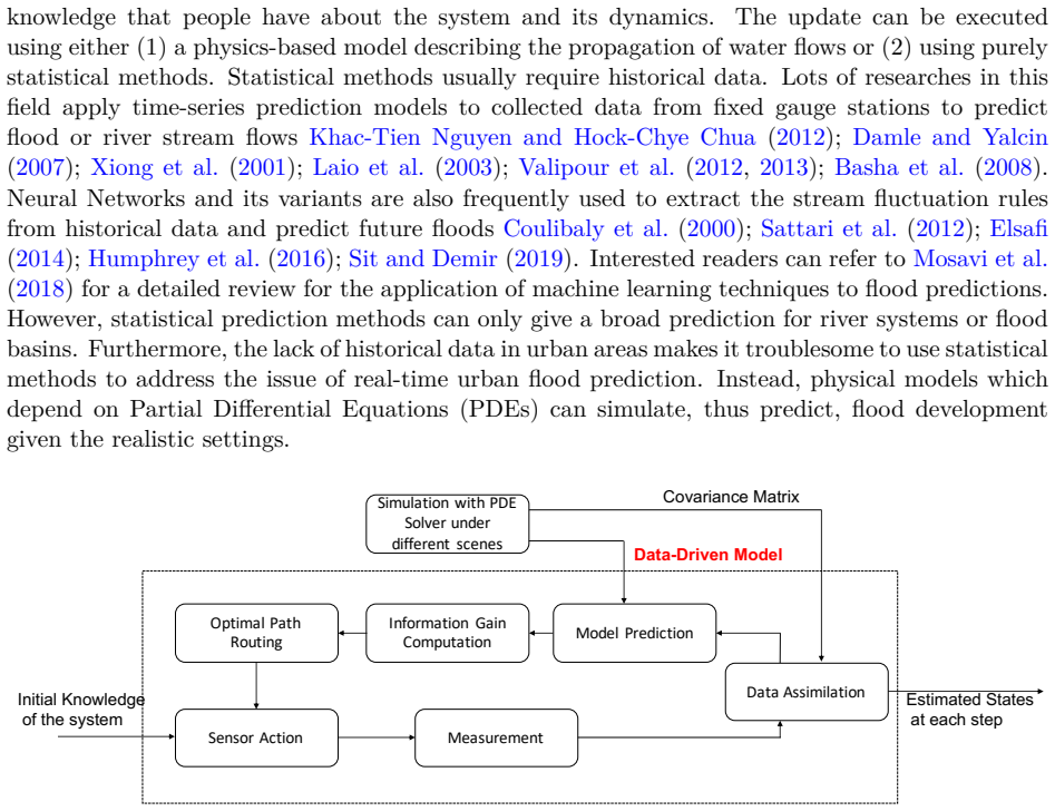
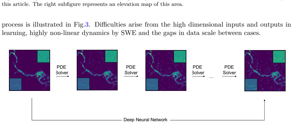
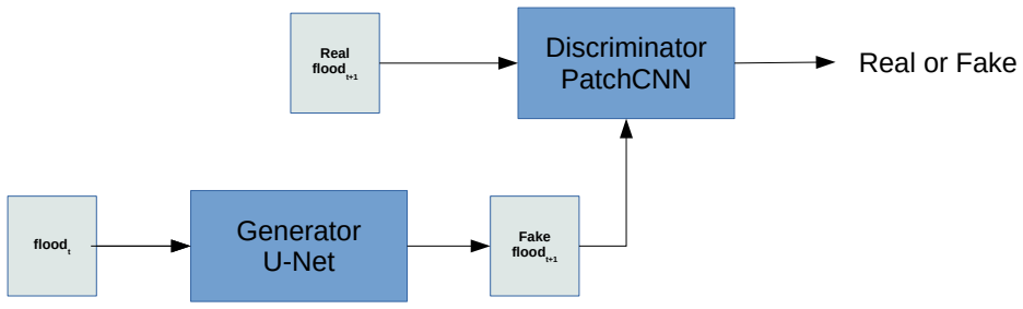
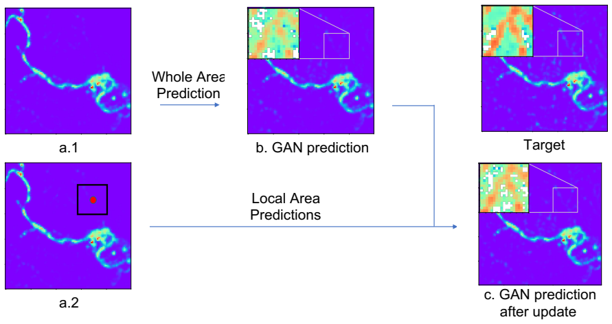
The central object is a Markovian leap map: because the shallow-water equations are first-order in time, the full state at time $t$ (water depth $h$, $x$-momentum $uh$, $y$-momentum $vh$) plus the next 30 minutes of rainfall and inflow determines the state at $t+30$; the paper replaces the PDE solver's many small time steps with a single convolutional network $\Phi$ that approximates this map. The network uses an encoder-decoder built from residual blocks, with $5\times100\times100$ input channels and $3\times100\times100$ output channels, and is trained with an $L^1$ loss; the best performer adds noise to inputs during training so that small errors made in a rollout do not compound. A secondary mechanism is the assimilation step: a Kalman-filter-style measurement update $\hat{X}=X+PH^T(HPH^T+R)^{-1}(z-HX)$ merges a global prediction with sparse local predictions to correct drift in generative models.
What would settle it
Hold out a disjoint set of simulations: train on snapshots from, say, 900 of the 1,080 simulations and test on the remaining 180, then compare the CNN rollout against the PDE solver on those unseen rainfall and inflow scenarios. If the error on unseen simulations is much larger than the reported validation MSE, the model has memorized training events rather than learned the shallow-water dynamics, and the real-time prediction claim fails.
Extended reading notes
Core claim
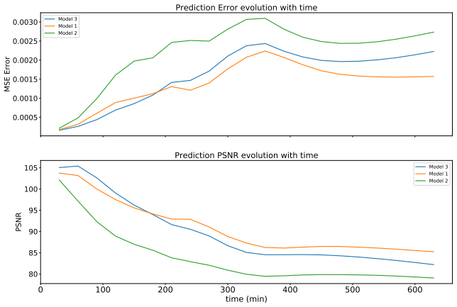
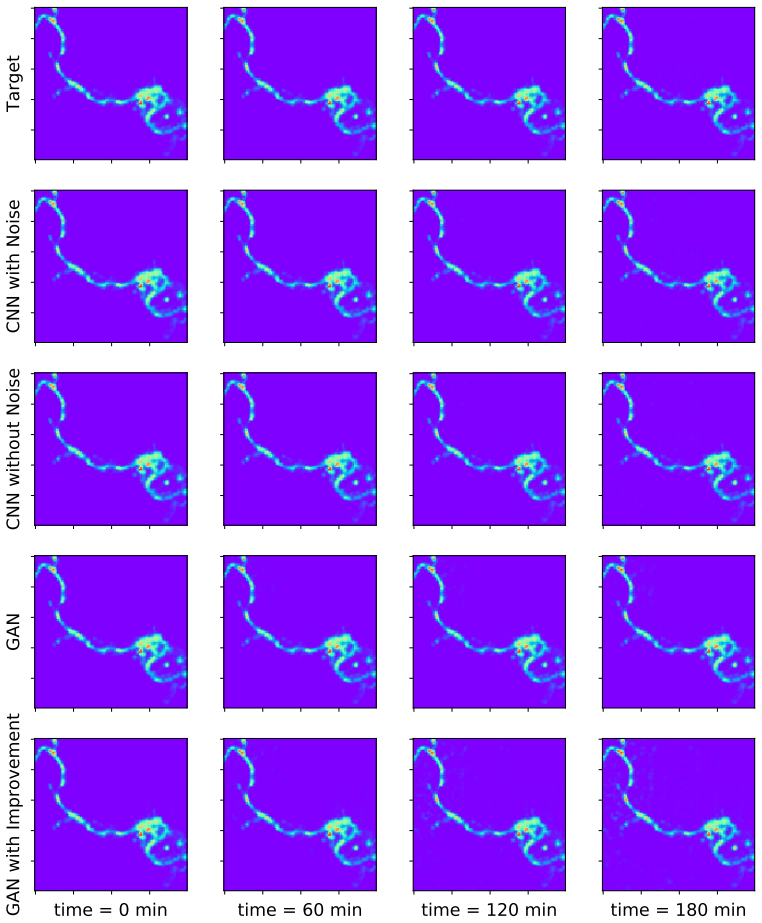
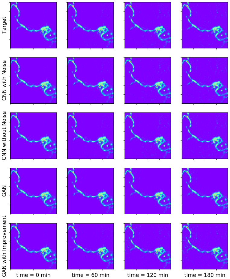
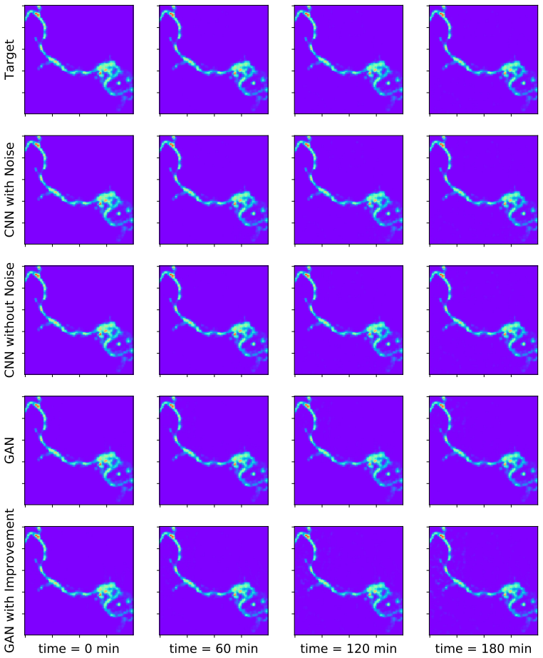
On the paper's own terms, the discovery is that the dynamics of the two-dimensional shallow-water equations, in a realistic urban watershed with rainfall and river inflow forcing, can be learned by a residual-block CNN from simulation data well enough that the network reproduces the solver's future states with low mean-squared error and stable PSNR over several hours of rolled-out prediction. A one-step prediction 30 minutes ahead takes one forward pass; the same CPU that needs hours to run the PDE solver executes it about 50,000 times faster. The authors further show that injecting noise during training stabilizes the multi-step temporal rollout, and that a measurement-update step in the style of the Kalman filter can pull a drifting generative model back toward the true state when sparse local observations are available.
Load-bearing premise
The load-bearing premise is that the validation pairs measure generalization to new floods; if the 2,000 validation snapshots are instead drawn from the same 1,080 simulations as the training snapshots, the reported error may mostly reflect memory of those specific events.
Editorial extensions
If this is right
- A trained CNN can replace the PDE solver in the forward-prediction step of a real-time flood monitoring loop, cutting the cost of a 30-minute city-wide forecast from minutes or hours to milliseconds on the same hardware.
- Because the surrogate is fast and its runtime is stable, ensemble data-assimilation methods such as the Ensemble Kalman Filter, which need many forward simulations, become computationally affordable for urban flood estimation.
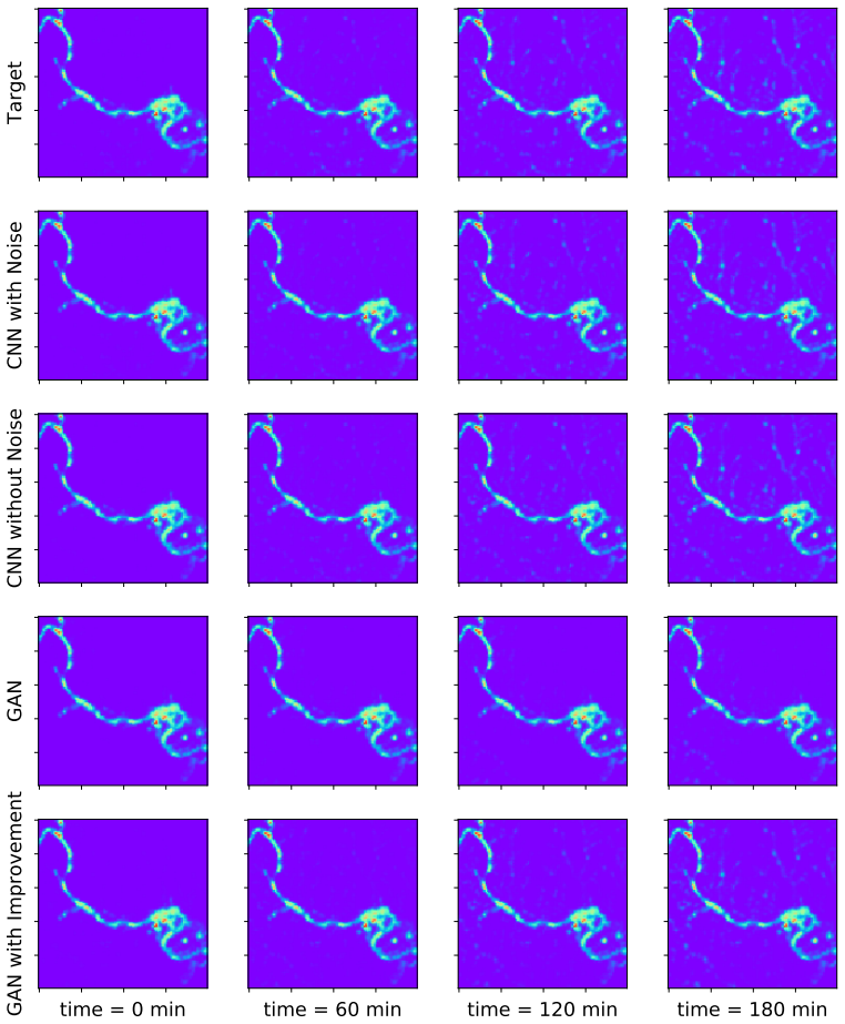
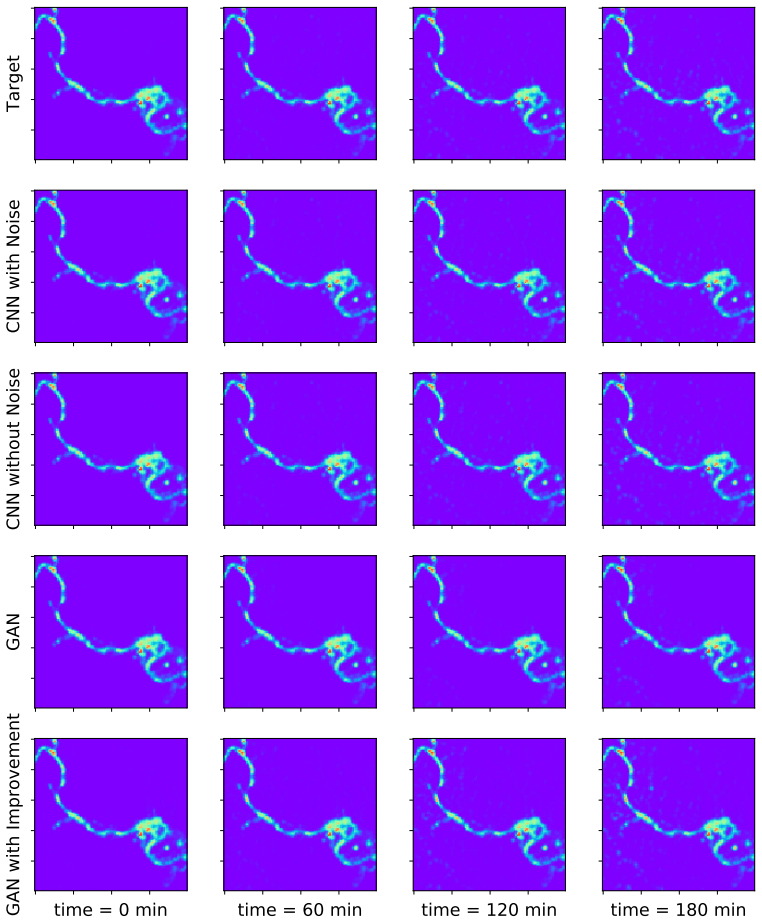
- Rolled-out CNN predictions stay close to the solver for several hours when the network is trained with input noise, so the model can serve not only one-step nowcasting but multi-step trajectory prediction.
- For cGAN-based models, the paper's Kalman-filter-style correction using sparse local predictions provides a way to keep long-horizon forecasts from diverging.
- The model outputs complete 100-by-100 fields of depth and momentum, so warnings can be localized to creeks, channels and streets rather than reduced to river-gauge readings.
Reading between the lines
- The pipeline is not tied to floods: the same recipe, letting a PDE solver generate snapshot pairs and training a residual CNN to learn the one-leap map, should transfer to other hyperbolic transport models such as storm surge, tsunami runup, or overland debris flow, provided enough simulations can be run.
- The strongest open test is the one the paper does not report: whether the network generalizes to rainfall and inflow patterns outside the 1,080 simulated configurations; this is what would decide whether a deployed system could be trusted before a novel storm.
- The soil, sewer, and building simplifications mean the surrogate inherits the solver's idealizations; pairing the network with the measurement-update step and real sensor data is a natural path toward closing that gap.
- The 50,000x speedup invites a swap of effort: spend more compute offline to train on finer meshes or more scenarios, since the online cost is a single forward pass.
Signed reviews
Editorial analysis
A structured set of objections, weighed in public.
Referee Report
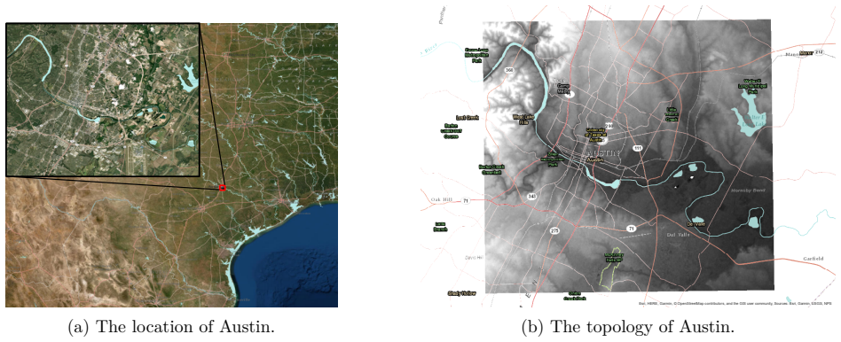
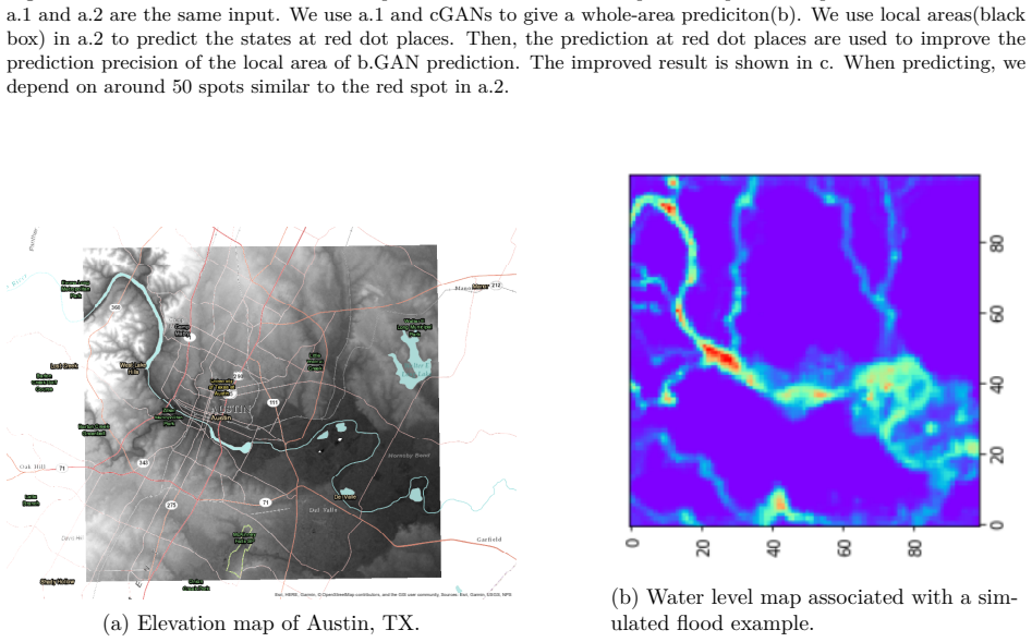
Summary. The manuscript proposes a data-driven surrogate for 2D shallow-water-equation flood simulation in an urban area (Austin, TX). CNN and conditional GAN models are trained on 10,000 input-output pairs extracted from 1,080 ANUGA simulations, with 2,000 pairs held out as validation; each pair maps a 5-channel 100x100 input (water depth, x- and y-momentum, expected inflow, expected precipitation) at time t to a 3-channel output at t+30 minutes. The authors report MSE and PSNR metrics, a temporal-evolution study over 30 time series, an assimilation step inspired by the Kalman filter, and a roughly 50,000x speedup compared with the PDE solver. The central claim is that the model provides precise real-time predictions of flood development that can replace the solver.
Significance. If the generalization claims were established, the work would be a valuable step toward real-time city-scale flood forecasting: it attacks a real operational bottleneck, compares several deep architectures, and makes code and data available. The strongest concrete contributions are the detailed architecture description, the comparison of CNN, cGAN, and an assimilation-augmented model, and the reproducible simulation-data pipeline. However, the current validation design does not demonstrate that the model predicts unseen rain/inflow scenarios, so the headline claims of 'precise' and 'real-time' predictions remain unsubstantiated for novel events.
major comments (4)
- [Section 3, Data Preparation] The validation set is not split by simulation. The text says that 'a stored result is randomly taken as an input' and 10,000/2,000 pairs are extracted, but it never states that validation pairs come from simulations absent from the training set. Because a simulation's internal states are highly correlated over time and share the same forcing pattern, random pairing can let the network memorize scenario-specific features rather than learn SWE dynamics. This directly affects the central claim of prediction for new flood events. The authors must split the 1,080 simulations into disjoint training/validation subsets (and preferably test on unseen forcing and boundary-condition combinations) and report the error on those held-out simulations.
- [Section 4.2, Temporal evolution] The temporal-evolution evaluation over '30 different pieces of time series data' does not state whether these series originate from simulations excluded from training. If they do not, the plotted MSE/PSNR curves and the statement that predictions 'align well' with the SWE results do not establish stability or accuracy for previously unseen scenarios. The same holdout-by-simulation discipline should be applied here.
- [Table 3 and Section 4.1] The 50,000x speedup claim is not fully documented. The caption states the PDE solver speed is averaged over 'a large number of different cases,' but the text does not report how the PDE time was measured, whether the comparison covers the same 30-minute prediction horizon, or whether the deep model time includes input preprocessing and output postprocessing. Without these details the speedup factor, which is a core part of the real-time claim, is not reproducible. Model 5's 10x figure suggests the assimilation step alone changes the comparison considerably; the measurement protocol should be described precisely.
- [Abstract and Section 1] The term 'physics informed' is used throughout, but the models do not incorporate the PDE residuals in the loss or architecture; they are trained purely on simulator output. This is not an error in itself, but the terminology overstates the connection to the governing equations. More importantly, no comparison to real-world flood observations is provided, so the 'precise' claim rests entirely on agreement with the training simulator. The authors should qualify the claims or add a clearly labeled discussion of this surrogate-validation limitation.
minor comments (6)
- [Equation (2.1)] Equation (2.1) is malformed: ∂U/∂t + h F = S does not correctly represent a conservation law; the typesetting should be fixed.
- [Appendix, GAN training] The authors use 'sued RMSprop' in the GAN training details; this should be 'used RMSprop'.
- [Conclusion and Abstract] The Conclusion lists important omitted processes (soil saturation, sewers, building impacts), but these limitations are absent from the Abstract and Introduction, where the model is described as 'precise'; the authors should align the claims with the enumerated simplifications.
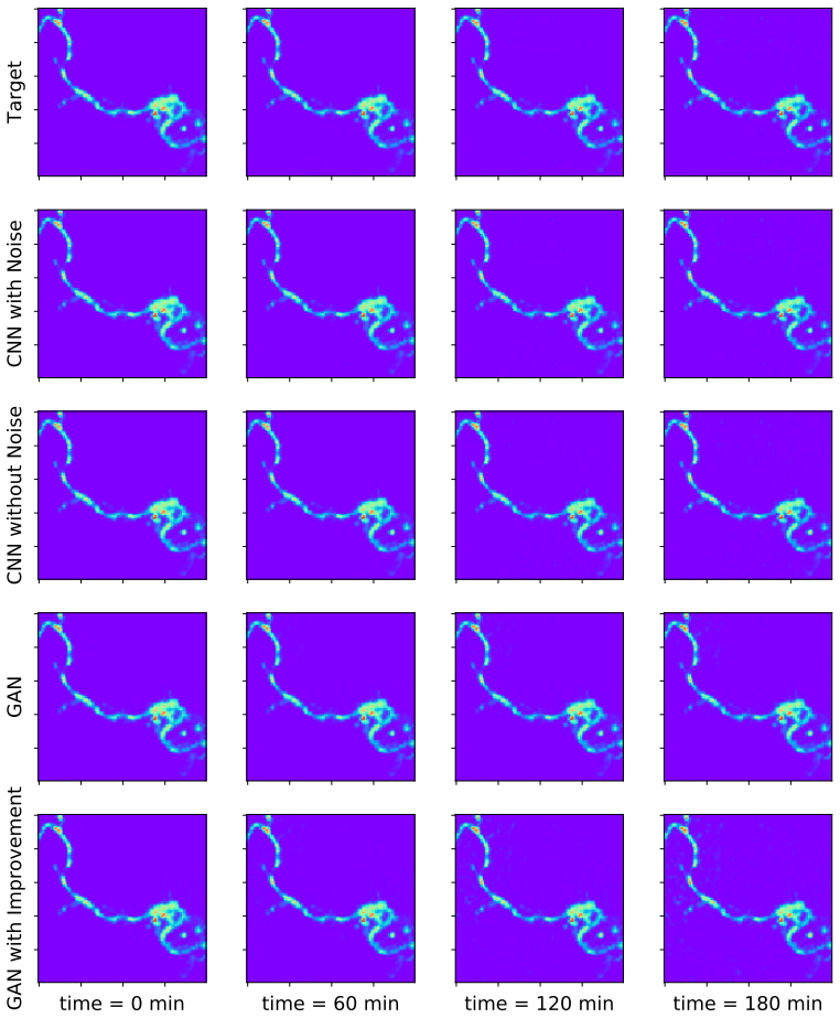
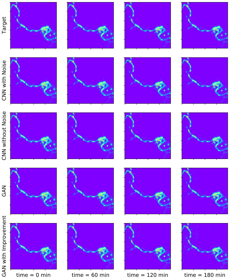
- [Appendix, additional illustrations] The appendix repeats the same four-panel comparison figures (Figures 16–26) without additional analysis; consider reducing redundancy or adding quantitative per-case metrics.
- [Section 2.2] The notation refers to '3 channels each pixel,' but the input has 5 channels; clarify.
- [Section 4.1] The MSE and PSNR values in Tables 1 and 2 are reported without confidence intervals or repeated-run variation; given the large number of training epochs, a single run may not be representative.
Circularity Check
No circularity found: the network is a surrogate trained on output of an independent PDE solver and evaluated on held-out simulated states.
full rationale
The paper's derivation chain is not circular. The deep learning models are trained on input/output pairs generated by ANUGA, an open-source finite-volume SWE solver (Section 3), so the training signal is external to the neural network. The inputs (water depth, momentum, expected inflow and precipitation) and outputs (simulated states 30 minutes later) are both defined directly from the PDE simulation, and no solver parameter or physical constant is fitted from the network's predictions. The reported MSE, PSNR, temporal-evolution curves, and speedup comparisons evaluate whether the learned map reproduces the solver's output on validation and test cases; they do not assert that the solver's physics is derived from the network. The claim that the data-driven model 'recovers the dynamics encoded by the 2D SWE' is a shorthand for learning a fast approximation of the solver, not a derivation of SWE from the model. No load-bearing self-citation or imported uniqueness theorem is used. The reviewer's concern about random train/validation pair splitting without simulation-level holdout is a real external-validity limitation for generalization to unseen flood scenarios, but it is a data-splitting weakness, not circularity: even with overlapping scenario memory, the target values remain independent solver outputs rather than functions of the model's own predictions.
Assumptions & free parameters
free parameters (4)
- Prediction horizon =
30 minutes
- L1 loss weight for GAN models =
not specified precisely
- Empirical covariance matrices P and R in assimilation =
not specified
- K-Means classes for river/channel/land =
3 classes
assumptions (5)
- domain assumption The 2D Shallow Water Equations accurately model urban flood dynamics
- domain assumption The Markov property holds for the discretized system
- domain assumption ANUGA solves the SWE accurately enough to serve as ground truth
- domain assumption The 1,080 simulated scenarios cover the diversity of real urban floods
- domain assumption Rain rate and river inflow for the next 30 minutes are known
Cite this review
Pith. "Pith review of Physics Informed Data Driven model for Flood Prediction: Application of Deep Learning in prediction of urban flood development." pith.science (2026). https://pith.science/paper/JANNC3ZA
@misc{pith2026190810312,
  author       = {Pith},
  title        = {Pith review of: Physics Informed Data Driven model for Flood Prediction: Application of Deep Learning in prediction of urban flood development},
  year         = {2026},
  howpublished = {\url{https://pith.science/paper/JANNC3ZA}},
  note         = {Machine review of arXiv:1908.10312}
}
read the original abstract
Flash floods in urban areas occur with increasing frequency. Detecting these floods would greatlyhelp alleviate human and economic losses. However, current flood prediction methods are eithertoo slow or too simplified to capture the flood development in details. Using Deep Neural Networks,this work aims at boosting the computational speed of a physics-based 2-D urban flood predictionmethod, governed by the Shallow Water Equation (SWE). Convolutional Neural Networks(CNN)and conditional Generative Adversarial Neural Networks(cGANs) are applied to extract the dy-namics of flood from the data simulated by a Partial Differential Equation(PDE) solver. Theperformance of the data-driven model is evaluated in terms of Mean Squared Error(MSE) andPeak Signal to Noise Ratio(PSNR). The deep learning-based, data-driven flood prediction modelis shown to be able to provide precise real-time predictions of flood development
Figures
Figures from the paper (21 more)








Reference graph
Works this paper leans on
-
[1]
A high-resolution godunov-type scheme in finite volumes for the 2d shallow-water equations
Alcrudo, F., Garcia-Navarro, P., 1993. A high-resolution godunov-type scheme in finite volumes for the 2d shallow-water equations. International Journal for Numerical Methods in Fluids 16 (6), 489--505
work page 1993
-
[2]
R., Natalizio, E., Calafate, C
Alvear, O., Zema, N. R., Natalizio, E., Calafate, C. T., 2017. Using uav-based systems to monitor air pollution in areas with poor accessibility. Journal of Advanced Transportation 2017
work page 2017
-
[3]
Anastasiou, K., Chan, C., 1997. Solution of the 2d shallow water equations using the finite volume method on unstructured triangular meshes. International Journal for Numerical Methods in Fluids 24 (11), 1225--1245
work page 1997
- [4]
-
[5]
Bai, S., Kolter, J. Z., Koltun, V., 2018. An empirical evaluation of generic convolutional and recurrent networks for sequence modeling. arXiv preprint arXiv:1803.01271
arXiv 2018
-
[6]
Basha, E. A., Ravela, S., Rus, D., 2008. Model-based monitoring for early warning flood detection. In: Proceedings of the 6th ACM conference on Embedded network sensor systems. ACM, pp. 295--308
work page 2008
-
[7]
Bellos, V., Tsakiris, G., 2016. A hybrid method for flood simulation in small catchments combining hydrodynamic and hydrological techniques. Journal of hydrology 540, 331--339
work page 2016
-
[8]
Recursive bayesian estimation: Navigation and tracking applications
Bergman, N., 1999. Recursive bayesian estimation: Navigation and tracking applications. Ph.D. thesis, Link \"o ping University
work page 1999
Show all 65 references
-
[9]
Flood disasters: lessons from the past—worries for the future
Berz, G., 2000. Flood disasters: lessons from the past—worries for the future. In: Proceedings of the Institution of Civil Engineers-Water and Maritime Engineering. Vol. 142. Thomas Telford Ltd, pp. 3--8
2000
-
[10]
A well-balanced reconstruction of wet/dry fronts for the shallow water equations
Bollermann, A., Chen, G., Kurganov, A., Noelle, S., 2013. A well-balanced reconstruction of wet/dry fronts for the shallow water equations. Journal of Scientific Computing 56 (2), 267--290
2013
-
[11]
The validity of flow approximations when simulating catchment-integrated flash floods
Bout, B., Jetten, V., 2018. The validity of flow approximations when simulating catchment-integrated flash floods. Journal of hydrology 556, 674--688
2018
-
[12]
R., S tra, M
Brodtkorb, A. R., S tra, M. L., Altinakar, M., 2012. Efficient shallow water simulations on gpus: Implementation, visualization, verification, and validation. Computers & Fluids 55, 1--12
2012
-
[13]
Data-driven synthesis of smoke flows with cnn-based feature descriptors
Chu, M., Thuerey, N., 2017. Data-driven synthesis of smoke flows with cnn-based feature descriptors. ACM Transactions on Graphics (TOG) 36 (4), 69
2017
-
[14]
Daily reservoir inflow forecasting using artificial neural networks with stopped training approach
Coulibaly, P., Anctil, F., Bobee, B., 2000. Daily reservoir inflow forecasting using artificial neural networks with stopped training approach. Journal of Hydrology 230 (3-4), 244--257
2000
-
[15]
\"U ber die partiellen differenzengleichungen der mathematischen physik
Courant, R., Friedrichs, K., Lewy, H., 1928. \"U ber die partiellen differenzengleichungen der mathematischen physik. Mathematische annalen 100 (1), 32--74
1928
-
[16]
Flood prediction using time series data mining
Damle, C., Yalcin, A., 2007. Flood prediction using time series data mining. Journal of Hydrology 333 (2-4), 305--316
2007
-
[17]
Generating images with perceptual similarity metrics based on deep networks
Dosovitskiy, A., Brox, T., 2016. Generating images with perceptual similarity metrics based on deep networks. In: Advances in neural information processing systems. pp. 658--666
2016
-
[18]
Robots for environmental monitoring: Significant advancements and applications
Dunbabin, M., Marques, L., 2012. Robots for environmental monitoring: Significant advancements and applications. IEEE Robotics & Automation Magazine 19 (1), 24--39
2012
-
[19]
H., 2014
Elsafi, S. H., 2014. Artificial neural networks (anns) for flood forecasting at dongola station in the river nile, sudan. Alexandria Engineering Journal 53 (3), 655--662
2014
-
[20]
Flooding, vulnerability and coping strategies: local responses to a global threat
Few, R., 2003. Flooding, vulnerability and coping strategies: local responses to a global threat. Progress in Development Studies 3 (1), 43--58
2003
-
[21]
P., 1986
Georgakakos, K. P., 1986. A generalized stochastic hydrometeorological model for flood and flash-flood forecasting: 1. formulation. Water Resources Research 22 (13), 2083--2095
1986
-
[22]
Scaling and similarity in rough channel flows
Gioia, G., Bombardelli, F., 2001. Scaling and similarity in rough channel flows. Physical review letters 88 (1), 014501
2001
-
[23]
Generative adversarial nets
Goodfellow, I., Pouget-Abadie, J., Mirza, M., Xu, B., Warde-Farley, D., Ozair, S., Courville, A., Bengio, Y., 2014. Generative adversarial nets. In: Advances in neural information processing systems. pp. 2672--2680
2014
-
[24]
Deep residual learning for image recognition
He, K., Zhang, X., Ren, S., Sun, J., 2016. Deep residual learning for image recognition. In: Proceedings of the IEEE conference on computer vision and pattern recognition. pp. 770--778
2016
-
[25]
A., Konev, A., Bl \"o schl, G., 2015
Horv \'a th, Z., Waser, J., Perdig \ a o, R. A., Konev, A., Bl \"o schl, G., 2015. A two-dimensional numerical scheme of dry/wet fronts for the saint-venant system of shallow water equations. International Journal for Numerical Methods in Fluids 77 (3), 159--182
2015
-
[26]
B., Gibbs, M
Humphrey, G. B., Gibbs, M. S., Dandy, G. C., Maier, H. R., 2016. A hybrid approach to monthly streamflow forecasting: integrating hydrological model outputs into a bayesian artificial neural network. Journal of Hydrology 540, 623--640
2016
-
[27]
E., 1960
Kalman, R. E., 1960. A new approach to linear filtering and prediction problems. Journal of basic Engineering 82 (1), 35--45
1960
-
[28]
The data-driven approach as an operational real-time flood forecasting model
Khac-Tien Nguyen, P., Hock-Chye Chua, L., 2012. The data-driven approach as an operational real-time flood forecasting model. Hydrological Processes 26 (19), 2878--2893
2012
-
[29]
P., Ba, J., 2014
Kingma, D. P., Ba, J., 2014. Adam: A method for stochastic optimization. arXiv preprint arXiv:1412.6980
2014 arXiv
-
[30]
V., Shirshov, G., Melnikova, N., Belleman, R
Krzhizhanovskaya, V. V., Shirshov, G., Melnikova, N., Belleman, R. G., Rusadi, F., Broekhuijsen, B., Gouldby, B., Lhomme, J., Balis, B., Bubak, M., et al., 2011. Flood early warning system: design, implementation and computational modules. Procedia Computer Science 4, 106--115
2011
-
[31]
Central-upwind schemes for the saint-venant system
Kurganov, A., Levy, D., 2002. Central-upwind schemes for the saint-venant system. ESAIM: Mathematical Modelling and Numerical Analysis 36 (3), 397--425
2002
-
[32]
Semidiscrete central-upwind schemes for hyperbolic conservation laws and hamilton--jacobi equations
Kurganov, A., Noelle, S., Petrova, G., 2001. Semidiscrete central-upwind schemes for hyperbolic conservation laws and hamilton--jacobi equations. SIAM Journal on Scientific Computing 23 (3), 707--740
2001
-
[33]
A second-order well-balanced positivity preserving central-upwind scheme for the saint-venant system
Kurganov, A., Petrova, G., et al., 2007. A second-order well-balanced positivity preserving central-upwind scheme for the saint-venant system. Communications in Mathematical Sciences 5 (1), 133--160
2007
-
[34]
A comparison of nonlinear flood forecasting methods
Laio, F., Porporato, A., Revelli, R., Ridolfi, L., 2003. A comparison of nonlinear flood forecasting methods. Water Resources Research 39 (5)
2003
-
[35]
Deep learning
LeCun, Y., Bengio, Y., Hinton, G., 2015. Deep learning. nature 521 (7553), 436
2015
-
[36]
Gradient-based learning applied to document recognition
LeCun, Y., Bottou, L., Bengio, Y., Haffner, P., et al., 1998. Gradient-based learning applied to document recognition. Proceedings of the IEEE 86 (11), 2278--2324
1998
-
[37]
Combining markov random fields and convolutional neural networks for image synthesis
Li, C., Wand, M., 2016. Combining markov random fields and convolutional neural networks for image synthesis. In: Proceedings of the IEEE Conference on Computer Vision and Pattern Recognition. pp. 2479--2486
2016
-
[38]
Numerical resolution of well-balanced shallow water equations with complex source terms
Liang, Q., Marche, F., 2009. Numerical resolution of well-balanced shallow water equations with complex source terms. Advances in water resources 32 (6), 873--884
2009
-
[39]
Some methods for classification and analysis of multivariate observations
MacQueen, J., et al., 1967. Some methods for classification and analysis of multivariate observations. In: Proceedings of the fifth Berkeley symposium on mathematical statistics and probability. Vol. 1. Oakland, CA, USA, pp. 281--297
1967
-
[40]
Conditional generative adversarial nets
Mirza, M., Osindero, S., 2014. Conditional generative adversarial nets. arXiv preprint arXiv:1411.1784
2014 arXiv
-
[41]
Uavs for smart cities: Opportunities and challenges
Mohammed, F., Idries, A., Mohamed, N., Al-Jaroodi, J., Jawhar, I., 2014. Uavs for smart cities: Opportunities and challenges. In: 2014 International Conference on Unmanned Aircraft Systems (ICUAS). IEEE, pp. 267--273
2014
-
[42]
E., Gruntfest, E., 2002
Montz, B. E., Gruntfest, E., 2002. Flash flood mitigation: recommendations for research and applications. Global Environmental Change Part B: Environmental Hazards 4 (1), 15--22
2002
-
[43]
RFFS and HYRAD: Integrated systems for rainfall and river flow forecasting in real-time and their application in Yorkshire
Moore, R., Jones, D., Black, K., Austin, R., Carrington, D., Tinnion, M., Akhondi, A., 1994. RFFS and HYRAD: Integrated systems for rainfall and river flow forecasting in real-time and their application in Yorkshire
1994
-
[44]
Flood prediction using machine learning models: Literature review
Mosavi, A., Ozturk, P., Chau, K.-w., 2018. Flood prediction using machine learning models: Literature review. Water 10 (11), 1536
2018
-
[45]
Deep hidden physics models: Deep learning of nonlinear partial differential equations
Raissi, M., 2018. Deep hidden physics models: Deep learning of nonlinear partial differential equations. The Journal of Machine Learning Research 19 (1), 932--955
2018
-
[46]
E., 2017 a
Raissi, M., Perdikaris, P., Karniadakis, G. E., 2017 a . Physics informed deep learning (part i): Data-driven solutions of nonlinear partial differential equations. arXiv preprint arXiv:1711.10561
2017 arXiv
-
[47]
E., 2017 b
Raissi, M., Perdikaris, P., Karniadakis, G. E., 2017 b . Physics informed deep learning (part ii): Data-driven discovery of nonlinear partial differential equations. arXiv preprint arXiv:1711.10566
2017 arXiv
-
[48]
Anuga user manual, release 2.0
Roberts, S., Nielsen, O., Gray, D., Sexton, J., Davies, G., 05 2015. Anuga user manual, release 2.0
2015
-
[49]
E., Hinton, G
Rumelhart, D. E., Hinton, G. E., Williams, R. J., et al., 1988. Learning representations by back-propagating errors. Cognitive modeling 5 (3), 1
1988
-
[50]
T., Yurekli, K., Pal, M., 2012
Sattari, M. T., Yurekli, K., Pal, M., 2012. Performance evaluation of artificial neural network approaches in forecasting reservoir inflow. Applied Mathematical Modelling 36 (6), 2649--2657
2012
-
[51]
R., 1996
Shewchuk, J. R., 1996. Triangle: Engineering a 2d quality mesh generator and delaunay triangulator. In: Workshop on Applied Computational Geometry. Springer, pp. 203--222
1996
-
[52]
Dgm: A deep learning algorithm for solving partial differential equations
Sirignano, J., Spiliopoulos, K., 2018. Dgm: A deep learning algorithm for solving partial differential equations. Journal of Computational Physics 375, 1339--1364
2018
-
[53]
Decentralized flood forecasting using deep neural networks
Sit, M., Demir, I., 2019. Decentralized flood forecasting using deep neural networks. arXiv preprint arXiv:1902.02308
2019 arXiv
-
[54]
Shallow water hydrodynamics: Mathematical theory and numerical solution for a two-dimensional system of shallow-water equations
Tan, W.-Y., 1992. Shallow water hydrodynamics: Mathematical theory and numerical solution for a two-dimensional system of shallow-water equations. Vol. 55. Elsevier
1992
-
[55]
Well, how accurate is it? a study of deep learning methods for reynolds-averaged navier-stokes simulations
Thuerey, N., Weissenow, K., Mehrotra, H., Mainali, N., Prantl, L., Hu, X., 2018. Well, how accurate is it? a study of deep learning methods for reynolds-averaged navier-stokes simulations. arXiv preprint arXiv:1810.08217
2018 arXiv
-
[56]
Accelerating eulerian fluid simulation with convolutional networks
Tompson, J., Schlachter, K., Sprechmann, P., Perlin, K., 2017 a . Accelerating eulerian fluid simulation with convolutional networks. In: ICML
2017
-
[57]
Accelerating eulerian fluid simulation with convolutional networks
Tompson, J., Schlachter, K., Sprechmann, P., Perlin, K., 2017 b . Accelerating eulerian fluid simulation with convolutional networks. In: Proceedings of the 34th International Conference on Machine Learning-Volume 70. JMLR. org, pp. 3424--3433
2017
-
[58]
E., Behbahani, S
Valipour, M., Banihabib, M. E., Behbahani, S. M. R., 2012. Parameters estimate of autoregressive moving average and autoregressive integrated moving average models and compare their ability for inflow forecasting. J Math Stat 8 (3), 330--338
2012
-
[59]
E., Behbahani, S
Valipour, M., Banihabib, M. E., Behbahani, S. M. R., 2013. Comparison of the arma, arima, and the autoregressive artificial neural network models in forecasting the monthly inflow of dez dam reservoir. Journal of hydrology 476, 433--441
2013
-
[60]
B., 2013
Vreugdenhil, C. B., 2013. Numerical methods for shallow-water flow. Vol. 13. Springer Science & Business Media
2013
-
[61]
Latent-space physics: Towards learning te temporal evolution of fluid flow
Wiewel, S., Becher, M., Th \"u rey, N., 2018. Latent-space physics: Towards learning te temporal evolution of fluid flow. CoRR abs/1802.10123
2018 arXiv
-
[62]
tempogan: A temporally coherent, volumetric gan for super-resolution fluid flow
Xie, Y., Franz, E., Chu, M., Thuerey, N., 2018. tempogan: A temporally coherent, volumetric gan for super-resolution fluid flow. ACM Transactions on Graphics (TOG) 37 (4), 95
2018
-
[63]
Y., O'connor, K
Xiong, L., Shamseldin, A. Y., O'connor, K. M., 2001. A non-linear combination of the forecasts of rainfall-runoff models by the first-order takagi--sugeno fuzzy system. Journal of hydrology 245 (1-4), 196--217
2001
-
[64]
Markov flow models and the flood warning problem
Yakowitz, S., 1985. Markov flow models and the flood warning problem. Water Resources Research 21 (1), 81--88
1985
-
[65]
Catastrophic collapse of water supply reservoirs in urban areas
Zoppou, C., Roberts, S., 1999. Catastrophic collapse of water supply reservoirs in urban areas. Journal of Hydraulic Engineering 125 (7), 686--695
1999
Reviewed August 14, 2026 · model on record in the stance chip above.
Discussion (0). Continue with ORCID to comment.