Learning Implicit Causal World Models from Multi-Agent Demonstrations

Jasorsi Ghosh

REVIEW 3 major objections 4 minor 13 references

Learning Implicit Causal World Models from Multi-Agent Demonstrations

T0 review · 3 major / 4 minor · reviewed 2026-08-01 · deepseek-v4-flash

Challenge this review Re-run · record.json Download PDF Read on arXiv ↗

Pith's one-line read The paper claims that the physical transition rules of a multi-agent environment can be recovered from purely observational demonstrations, without hand-specified causal graphs, provided the demonstrations mix expert behavior with controlle

desk verdict A self-aware empirical study of soft interventions for multi-agent world models, whose formal identifiability theorem rests on assumptions the paper asserts but never validates. read the letter →

arxiv 2607.26336 v1 pith:JBIVZW7N submitted 2026-07-28 cs.LG cs.MAcs.RO

Jasorsi Ghosh This is my paper

classification cs.LGcs.MAcs.RO

keywords causalworldmodelsmulti-agentreinforcementlearningsequentialbackdoorconditionsoftinterventionspolicyvarianceofflinedemonstrationsdiscoveryout-of-distributionrobustness

verification ladder T0 review T1 audit T2 compute T3 formal

The pith

A machine-rendered reading of the paper's core claim, the machinery that carries it, and where it could break.

The reading

This paper tries to establish that environmental physics—the invariant rules governing how states change in response to joint actions—can be disentangled from hidden strategic intent in multi-agent systems using only offline demonstrations. The key move is injecting controlled randomness into agent policies during data collection, which the authors formalize as a soft intervention satisfying a new Multi-Agent Sequential Backdoor Condition. If correct, this means causal world models can be learned without costly hard interventions or predefined causal graphs, and model accuracy and out-of-distribution transfer improve as the injected randomness (interventional strength) grows. A sympathetic reader would care because it offers a practical path toward robust, interpretable world models for autonomous systems operating alongside other agents.

What carries the argument

The central object is the Multi-Agent Sequential Backdoor Condition (Theorem 1), a do-calculus adjustment formula that makes interventional transitions computable from observational distributions by marginalizing over peer actions. It is carried by three working parts: (1) a soft-intervention data collection scheme using a stationary policy mixture P^σ(a|s) = (1−σ)π^exp(a|s) + σζ(a); (2) the PCMCI+ algorithm to discover the lagged causal skeleton, discarding contemporaneous edges attributed to latent intent; and (3) a differentiable soft mask that restricts the neural transition model's receptive field to the discovered causal parents.

What would settle it

Collect a high-σ dataset in the Giveway or Navigation simulator, then apply hard interventions (clamp one agent's action to a fixed vector over many histories). Compare the measured interventional distribution against the Eq. (7) backdoor adjustment computed from the observational data. If the two differ significantly—especially in timesteps where collision-avoidance physics modifies one agent's action in response to the other's—the adjustment is biased and Theorem 1's identifiability claim collapses. A second check is to vary the history length τ used in the adjustment; if estimates shift sub

Watch

Extended reading notes

Core claim

The central discovery is that the interventional transition dynamics of one agent, P(s_{t+1} | do(a^i_t), H_k), are identifiable from observational multi-agent data through the sequential backdoor adjustment P(s_{t+1} | do(a^i_t), H_k) = Σ_{a^{-i}_t} P(s_{t+1} | a^i_t, a^{-i}_t, H_k) P(a^{-i}_t | H_k). This becomes evaluable only when the data contains policy variance, i.e., when actions are mixtures of expert behavior and an independent stochastic process. The paper proves this adjustment in a mutilated causal decision graph, establishes a generalization error bound scaling as 1/√(Nσ), and shows empirically that both recovered causal graph quality and out-of-distribution predictive accuracy

Load-bearing premise

The load-bearing premise is that the observed history H_k completely captures the latent strategic intent (so the next state is independent of intent given history and joint actions) and that agents' simultaneous actions do not directly cause each other; the paper asserts both without proof and does not verify them against its own simulators' integration steps.

Editorial extensions

If this is right

Offline multi-agent datasets with policy variance can yield causal world models without hard interventions or hand-specified causal graphs.
Recovered causal structure and one-step prediction accuracy improve as interventional strength σ grows, with adversarial out-of-distribution error falling by up to two orders of magnitude.
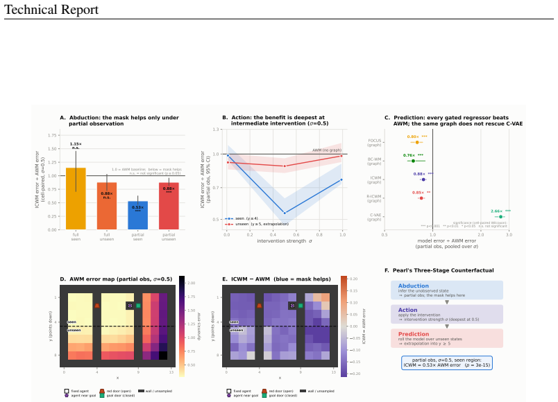
Graph quality and predictive accuracy are both driven by interventional strength as a common cause; the causal mask mainly adds value under partial observation and layout extrapolation, while a corrupted mask is worse than no mask at all.
The approach scales from two to four agents and generalizes across both fully and partially observable settings.
Soft interventions identify dynamics within a fixed geometry but do not enable spatial extrapolation to rearranged layouts; performance degrades when the layout changes.

Reading between the lines

Editorial extensions of the paper, not claims the author makes directly.

The adjustment formula suggests a broader principle: any offline multi-agent dataset containing at least two distinct action choices in near-identical states encodes enough information to estimate counterfactual action effects, potentially unlocking causal replay buffers for offline RL.
Given that graph quality contributes no predictive value beyond σ in well-sampled regimes, a testable extension is that the causal mask should provide larger gains in low-data regimes where σ cannot be raised.
The boundary result—σ helps within a geometry but not spatial rearrangement—mirrors the distinction between learning a function (dynamics) and its domain (coordinates); coupling ICWM with a geometry-adaptive coordinate mapping might extend identifiability to layout shifts.
The sufficiency-of-history assumption implies identifiability should degrade as history length shrinks in partially observable settings; this could be validated by ablating the recurrent memory depth in R-ICWM.

Share X Bluesky LinkedIn Reddit HN

Editorial analysis

A structured set of objections, weighed in public.

Desk editor's note, referee report, and a circularity audit.

Desk Editor's Note

read the letter

Dear colleague,

Quick take: the empirical core is more interesting than the theory, and the paper half-admits this. The headline claim—that interventional strength sigma makes world models identifiable and accurate—is overstated. The paper's own Two-Door results show no sigma trend in prediction error, and layout shifts invert the scaling. But the C5 analysis—that recovered-graph quality and OOD error are both driven by sigma as a common cause—is a genuinely useful negative result for the causal-world-model literature.

What's new: the multi-agent sequential backdoor adjustment (Eq. 7), conditioning on contemporaneous peer actions, is a legitimate extension of the standard backdoor criterion, even if it reduces to familiar ideas under a clear graph. The paper also ships a large, careful experimental map across three environments, full/partial observability, team sizes, and honest shifted-layout controls. The mask-corruption ablation and the uncertainty-localization analysis are well done. Credit where due: the authors report the counterexamples themselves rather than hiding them.

Where it gets soft: Theorem 1's proof in Appendix F depends on a 'Sufficiency of History' assumption (F.2) and a no-contemporaneous-coupling axiom (F.1) that are asserted, not proven or checked against the simulators. In VMAS, simultaneous actions interact through collision physics within the integration step; the paper never shows Axiom 2 holds there. If U has any direct effect on s_{t+1} beyond realized actions, Eq. (7) picks up an unidentified term. The stress-test note is right: the theorem's force is conditional on an assumption close to the conclusion. The generalization bound (Lemma 1) is generic and assumes discrete actions and uniform zeta; fine as a sketch, but it doesn't do the work the abstract implies.

The abstract says 'model accuracy scaling directly with interventional strength,' while Figure 39 shows Two-Door does not follow the trend. The dataset for Two-Door was collected at a looser tolerance (0.5 vs 0.1 std-dev), which muddies the one environment that breaks the pattern—a minor but real confound.

Who should read this: anyone working on causal discovery or world models for multi-agent RL, especially for the C5 common-cause point and the shifted-layout boundary. It deserves a serious referee; the theory needs revision or at least validation of its assumptions against the actual simulators, and the paper would benefit from releasing code and data. I'd send it to review, with the expectation that the theorem gets reworked or the claims toned down.

Best, [Your name]

Referee Report

3 major / 4 minor

Summary. The paper proposes Implicit Causal World Models (ICWM), a framework for recovering multi-agent environment transition dynamics from offline demonstrations by injecting stochastic soft interventions into the data-collection policy. The central theoretical claim is a Multi-Agent Sequential Backdoor Condition (MAS-SBC), Theorem 1, which states that the interventional transition P(s_{t+1}|do(a^i_t), H_k) is identifiable from observational data via Eq. (7), provided latent strategic intent is d-separated by history and peer actions. The empirical section evaluates the method on Two-Door, Navigation, and Giveway, under full and partial observability, with graph recovery, OOD transfer, uncertainty localization, mask ablations, and layout shifts. The paper also proposes a PAC-style generalization bound scaling as 1/sqrt(N sigma), and a series of claims about when causal masks help or hurt.

Significance. If the main identifiability theorem were established for the target simulators, this would be a meaningful step: it would show that policy variance in multi-agent demonstrations can act as a soft intervention, allowing environmental physics to be disentangled from unobserved strategic intent without costly hard interventions. The empirical design has notable strengths: comparisons against graph-free and ablation baselines, ground-truth causal graphs, controlled layout shifts, honest discussion of when the intervention lever stops working, and a reproducibility statement. However, the central theorem is formally conditional on assumptions that are asserted rather than derived or validated, and the empirical headline is partially contradicted by the paper's own Two-Door and layout-shift results. The contribution is therefore promising but not yet fully supported.

major comments (3)

[Appendix F.2 / Eq. (7)] The proof of Theorem 1 assumes the key d-separation fact it is supposed to establish. Axiom 1 in F.1 is exactly the 'Sufficiency of History' asserted in F.2, and the inductive proof's base case simply says that under sufficiency of history, H_k screens off U. Step 3 of F.3 then invokes Axiom 1 to drop U from the transition term. Thus Eq. (7) is a conditional algebraic identity, not a demonstration that MAS-SBC holds for the VMAS/MiniGrid environments used later. Since this theorem is the formal basis for C2 and the abstract's identifiability claim, the paper must either prove this sufficiency from the simulators' step functions or validate it empirically, e.g., by comparing Eq. (7) with oracle do-interventions in the three environments. This is load-bearing.
[Appendix H, Lemma 1] The proof of Lemma 1 assumes zeta is uniform over a discrete joint action space, giving min_a P_sigma(a|s) >= sigma/|A| in Eq. (14). But two of the three evaluation environments (Navigation and Giveway, Appendix M.1) use continuous action spaces in R^2. For continuous actions there is no positive lower bound of this form, and the constant J defined after Eq. (18) contains |A| and d_min in a way that is not meaningful for continuous action spaces. Consequently the quantitative 1/sqrt(N sigma) bound in Theorem 2 is not actually established for the flagship environments. The authors need a continuous-action concentration argument (e.g., a lower-bounded density and a different empirical-process bound), or the bound should be explicitly restricted to discrete-action settings.
[Figure 39 / Abstract] The abstract claims that 'evaluations across coordination tasks ... demonstrate ... model accuracy scaling directly with interventional strength.' The paper's own Figure 39 shows that Two-Door does not exhibit this trend: its error remains roughly flat across sigma, and the caption attributes this to the sparsity living in the input-output transition matrix. Moreover, Figure 4A shows that under layout rearrangements transfer error grows with sigma (1.9x to 5.3x), which is acknowledged in the conclusion but not reflected in the abstract or claim C3 as stated. The claim should be qualified as environment-dependent and separated into graph recovery, one-step accuracy, and OOD transfer. This is not a fatal flaw, but it is a mismatch between the headline and the data.

minor comments (4)

[General] There are numerous typos: 'enviornment', 'Giveaway' vs 'Giveway', 'NILL' instead of NLL, and several inconsistent references to appendices (e.g., the index lists 'Appendix E.3' while Appendix E already has E.3). A careful proofread is needed.
[Section 4.1] The sentence 'The complete formal proof (claim C5) using Pearl's do-calculus...' appears to be a mislabeling; the proof concerns Theorem 1/claim C2, not claim C5. Please correct the cross-reference.
[Table 16 / Section 4.4] The causal discovery is run with tau_max = 1, but the MAS-SBC theorem is stated with a general history H_k. The paper should state clearly whether the empirical results validate only the tau=1 instance, and how the identifiability argument extends to longer histories needed for POMDP settings.
[Appendix M.2] The MiniGrid action space description says 'The required dimension is effectively 1D', but the action table has 7 categorical values. This is fine, but the ambiguity between 'dimension' and 'support size' should be clarified.

Circularity Check

1 steps flagged · score 4.0 of 10

MAS-SBC identifiability theorem's key algebraic step is the assumed 'Sufficiency of History' (Axiom 1) itself, so Eq. (7) reduces by construction to the conditional-independence assumption; the abstract presents this conditional result as an achieved discovery.

self definitional [Appendix F.2–F.3 (proof of Theorem 1, Eq. 7 in §4.1); Abstract / Contribution C2]
"We require the assumption of Sufficiency of History: The observed history H_k acts as a sufficient statistic for the latent intent U, meaning s_{k+1} ⊥⊥ U | (H_k, a^i_k, a^{-i}_k). ... Applying Axiom 1: The transition is fully determined by observed variables. ... Thus, P(s_{t+1}|do(a^i_t), a^{-i}_t, H_k, U) = P(s_{t+1}|a^i_t, a^{-i}_t, H_k)."

F.3 Step 3's decisive equality — P(s_{t+1}|do(a^i_t),a^{-i}_t,H_k,U) = P(s_{t+1}|a^i_t,a^{-i}_t,H_k) — is exactly the 'Sufficiency of History' assumption (Axiom 1) that F.2 says 'We require'; substituting it yields Eq. (7) by construction. The theorem's conclusion is that assumed conditional independence restated as a backdoor adjustment. C2's 'recoverable ... despite unobserved strategic confounding' is guaranteed only because the axioms define U to have no direct effect on s_{t+1} given the adjustment variables; if persistent intent affected the transition beyond the realized action, Eq. (7) would carry the unidentified term Σ_U P(s_{t+1}|a^i,a^{-i},H,U)P(U|H). The abstract's unconditional 'we render world models discoverable' overstates the conditional theorem, and the axiom is never va

full rationale

The derivation chain is mostly transparent and non-circular: Theorem 2's generalization bound is a valid concentration-plus-Simulation-Lemma argument whose 1/√σ dependence is definitional to the mixture policy (Eq. 14, min P_σ(a|s) ≥ σ/|A|) rather than a fitted parameter renamed as a prediction; the empirical program (Figures 3, 35, 39) is self-contained, seeded, and honestly reports failures (Two-Door shows no σ-trend; layout shifts invert the trend). There is no load-bearing self-citation: the only author-overlapping reference (Deng et al., 2025, co-authored by Ghosh) is cited contextually alongside Arjovsky et al. for 'distributional shifts,' and no uniqueness theorem or ansatz is imported from the authors' prior work. The circularity concern is localized to the central theoretical claim. Theorem 1 (Eq. 7) is the standard backdoor adjustment with adjustment set {H_k, a^{-i}_t}, and its proof's load-bearing reduction (F.3 Step 3) is the unproven 'Sufficiency of History' axiom (F.2), which asserts exactly that U is irrelevant to s_{t+1} once history and the realized actions are conditioned on — i.e., that the confounding is removable. The conclusion is then entailed by construction, and the main text's theorem statement omits the appendix-only axioms, so the abstract's 'render world models discoverable via the sequential backdoor condition' presents a conditional result as an unconditional achievement. The assumption is neither derived from the SCM's own simulator step functions nor empirically validated (τ_max=1 in Table 16 would not capture a persistent planning variable; VMAS collision resolution inside a step would couple A^{-i} with A^i and give U a direct path to s_{t+1}), directly threatening the 'despite unobserved strategic confounding' claim. Score 4: partial circularity in the central identifiability claim, with independent and credible empirical content elsewhere.

Assumptions & free parameters 4 free parameters · 9 assumptions · 0 invented entities

The central claims rest on a large implicit burden: three structural axioms plus an unproven sufficiency assertion for Theorem 1, a temporal-lag assumption that justifies throwing away all contemporaneous discovery output, and a discrete-action uniformity assumption that contradicts the continuous experimental domains. The free parameters (σ, thresholds, ε_env) are hand-chosen and none are fitted, but ε_env is unestimated, making the headline bound unfalsifiable in practice.

free parameters (4)

σ (interventional strength) = swept {0.01, 0.25, 0.50, 0.75, 0.99}
Central design knob: mixture weight of random actions in Eq. (4). Not fitted, but both theorems and all empirical claims are functions of it; the paper never optimizes σ, treating it as an input.
Mask/discovery hyperparameters (α, pc_alpha, κ, τ) = α=0.005; pc_alpha=0.1; κ=1.0; τ=1
Chosen by hand in Appendices T.1/P.2; the soft-mask gate Γ and the discovered skeleton depend directly on these thresholds, and no sensitivity analysis is reported.
ε_env (irreducible error) = not estimated
Free slack term in Lemma 1's bound (Appendix H); it absorbs neural approximation error and is never quantified, so the bound can be made to hold for any observed error level.
Dataset tolerance thresholds = 0.5 std-dev (Two-Door); 0.1 std-dev (others)
Sample-cardinality tolerances chosen per environment (Appendix S.1, Table 13); the environment where the σ-trend fails (Two-Door) used the looser tolerance, putting it on a different data-quality footing.

assumptions (9)

domain assumption Transition Markovianity (Axiom 1): S_{t+1} ⊥⊥ U | (H_k, A^i_t, A^{-i}_t)
Appendix F.1. Declares the transition independent of latent intent given history and joint actions; in the paper's SCM (Eq. 1) this holds by construction, so it is built into the model rather than established.
domain assumption Decentralized policy (Axiom 2): A^i_t ⊥⊥ A^{-i}_t | (H_k, U)
Appendix F.1. Asserts no direct simultaneous coupling between agents' actions; never verified against the VMAS collision/avoidance step structure.
domain assumption Confounding structure (Axiom 3): U → A^i_t and U → A^{-i}_t
Appendix F.1. Postulates a shared latent intent driving all agents; standard but untestable from the demonstration data used.
ad hoc to paper Sufficiency of History (s_{k+1} ⊥⊥ U | H_k, a^i_k, a^{-i}_k)
Appendix F.2. Asserted without proof and load-bearing for the d-separation step of Theorem 1; if history is not sufficient, the MAS-SBC adjustment is biased.
domain assumption Strict temporal lag τ ≥ 1 (Assumption i, §4.4)
Used to discard all contemporaneous edges E_contemp as spurious; if any physical effect is instantaneous within a timestep, real dynamics are dropped from the skeleton.
domain assumption Contemporaneous confounding isolation (Assumption ii, §4.4)
u_intent coordinates actions only at time t with no lagged effect on s_{t+1}; needed so that E_contemp carries only spurious correlations.
ad hoc to paper ζ uniform over a discrete joint action space
Appendix H proof of Lemma 1; two of three experimental domains use continuous force actions, so the bound's assumptions do not cover the experiments.
domain assumption Ergodicity / d_min > 0 for the MDP
Appendix H Lemma 1; guarantees every state-action pair is visited with positive probability but is not checked for the three finite-horizon tasks.
standard math Faithfulness and noise independence for PCMCI+
Required by the MCI tests; the paper itself notes (Appendix T.4) that deterministic LiDAR couplings violate faithfulness, so the assumption is known to fail in one of its own setups.

how reviews work

0 comments

Cite this review

Pith. "Pith review of Learning Implicit Causal World Models from Multi-Agent Demonstrations." pith.science (2026). https://pith.science/paper/JBIVZW7N

@misc{pith2026260726336,
  author       = {Pith},
  title        = {Pith review of: Learning Implicit Causal World Models from Multi-Agent Demonstrations},
  year         = {2026},
  howpublished = {\url{https://pith.science/paper/JBIVZW7N}},
  note         = {Machine review of arXiv:2607.26336}
}

read the original abstract

In model-based reinforcement learning, world models exist as internal simulators, but their training often conflates statistical correlations with causal mechanisms. This problem is exacerbated in multi-agent systems where physical transitions are intertwined with strategic agent intents, causing world models to fail under distribution shift. We introduce Implicit Causal World Models to recover environmental dynamics from offline demonstrations without requiring pre-defined causal graphs. By incorporating policy variance, we render world models discoverable via the sequential backdoor condition. Evaluations across coordination tasks (Two-Door, Navigation, and Giveway) demonstrate that these models provide interpretable causal representations under both full and partial observability, with model accuracy scaling directly with interventional strength.

Figures

Figures reproduced from arXiv: 2607.26336 by the authors.

**Figure 1.** A learned causal dynamics transfers to states the model has never seen. The region below the dashed line is unseen in training. Full details in Appendix Z This challenge is compounded in multi-agent systems, where environmental physics are intertwined (Lowe et al., 2020; Dasgupta et al., 2019) with the strategic, often confounded, intents of other agents. For example, an autonomous vehicle model might incorrectly l… view at source ↗

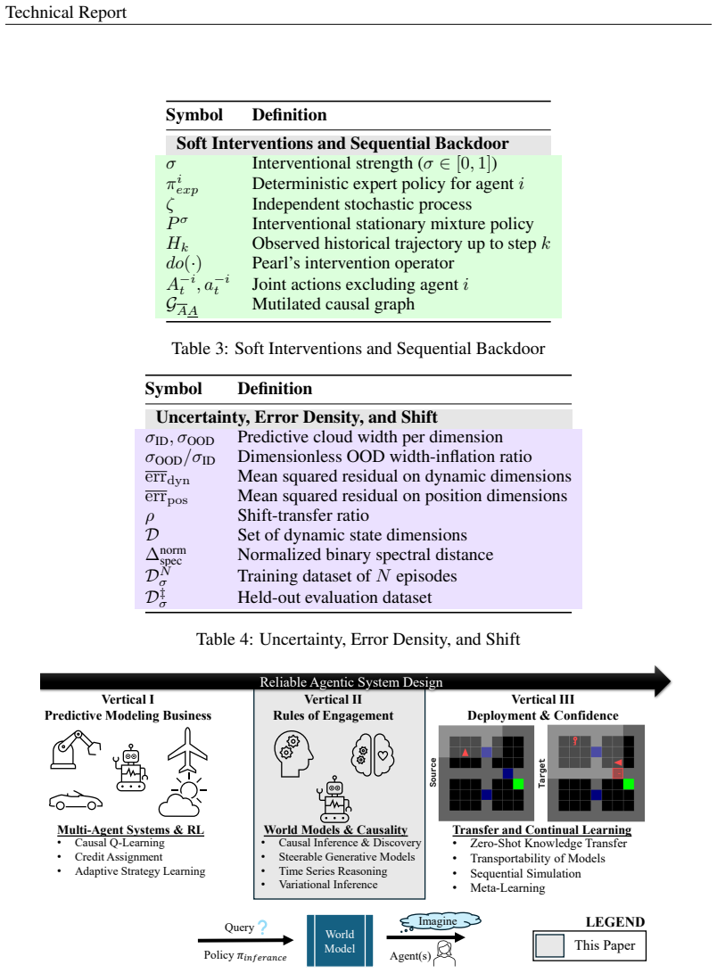
**Figure 2.** Overview of the ICWM Framework: (a) Stochastic Demonstrations: Expert multi-agent trajectories collected via soft interventions. (b) Feature Extraction: Temporal features (r, a, s) processed for causal discovery. (c) Causal Structure Discovery: Learned world model showing reward and transition physics across temporal lags (Lag 1: t−1 → t, Lag 2: t−2 → t). (d) Benchmarking: Stress testing under exploratory (πrandom)… view at source ↗

**Figure 3.** Interventional strength drives both causal-structure recovery and out-of-distribution transfer. (A) Graph error vs σ (dashed: navigation 2/3/4 agents). (B) Adversarial error (MSE/Var) vs σ. (C) Per-axis OOD/ID density-width inflation, dimensions sorted. (D) Adversarial error vs graph error; broken lines trace the σ = 0.99→0.01 trajectory. (E) σ lowers both errors together (common cause, not a direct link). Details i… view at source ↗

Figures from the paper (67 more)

**Figure 4.** Figure 4: What actually breaks a world model under shift, and what the mask is worth. (A) All seven shifted layouts on the dynamics/position plane, scored against each frozen model’s own error on the layout it trained on, so smaller is better. ρ= 1 is lossless and the green regi…

**Figure 5.** Figure 5: Velocity error, R-ICWM minus ICWM (log10). Below 0 means R-ICWM is better. Its edge grows as the trained speed of a region drops, in all three layouts (Source, Easy, Mirror). Being off-manifold is not automatically harder. What matters is whether the changed mechanism…

**Figure 6.** Figure 6: The Synergistic Vertical Framework for Reliable Agentic Systems. The architecture partitions system design into three critical pillars: behavioral coordination (Vertical I), structural understanding (Vertical II), and cross-domain scalability (Vertical III). This pape…

**Figure 7.** Figure 7: Causal Decision Graph for MAS (a) MDP (b) MDP with Confounding (c) Partially Ob [PITH_FULL_IMAGE:figures/full_fig_p022_7.png]

**Figure 8.** Figure 8: Navigation trajectories from source to goal for a single agent (left) and two agents (right). [PITH_FULL_IMAGE:figures/full_fig_p024_8.png]

**Figure 9.** Figure 9: Manipulated Causal Decision Graph for a single agent (a) MDP with SBC at [PITH_FULL_IMAGE:figures/full_fig_p025_9.png]

**Figure 10.** Figure 10: The dynamic confounding path in multi-agent systems. Contemporaneous actions ( [PITH_FULL_IMAGE:figures/full_fig_p026_10.png]

**Figure 11.** Figure 11: Mutilated Causal Decision Graph GAi for MAS-SBC Identifiability. The hammer indicates the intervention do(a i k ), which severs incoming edges from Hk and U. Conditioning on the intact peer actions (a −i k ) blocks the contemporaneous backdoor path. • Axiom 1: Transit…

**Figure 12.** Figure 12: Motivation study in Tic-Tac-Toe. (a) Environment representation with initial agent [PITH_FULL_IMAGE:figures/full_fig_p028_12.png]

**Figure 13.** Figure 13: Logic flowchart for Tic-Tac-Toe agent decision-making. Algorithm 1: Optimal Tic-Tac-Toe Move Selection 1: Input: Board state S, Player ID P 2: Output: Best action a ∈ LegalActions(S) 3: if ∃a ∈ LegalActions(S) completes line for P then 4: return a ▷ Win immediately 5…

**Figure 14.** Figure 14: Analysis of Optimal Policy Performance and Exploration Entropy. (a) Optimal policy [PITH_FULL_IMAGE:figures/full_fig_p030_14.png]

**Figure 15.** Figure 15: Model architectures and evaluation. (a) Schematic representation of various world mod [PITH_FULL_IMAGE:figures/full_fig_p031_15.png]

**Figure 16.** Figure 16: Causal discovery graph reconstruction comparison between the PC algorithm (blue, left [PITH_FULL_IMAGE:figures/full_fig_p032_16.png]

**Figure 17.** Figure 17: Out-of-distribution (OOD) performance analysis and model architecture. (a) OOD Test [PITH_FULL_IMAGE:figures/full_fig_p033_17.png]

**Figure 18.** Figure 18: Split violin plots comparing OOD Test MSE between ground truth causal masks (lighter [PITH_FULL_IMAGE:figures/full_fig_p035_18.png]

**Figure 19.** Figure 19: Failure mode: Winning and recovery. Density peaks under an adversarial intervention [PITH_FULL_IMAGE:figures/full_fig_p036_19.png]

**Figure 20.** Figure 20: Failure mode: Blocking and recovery. Density peaks when the agent is forced away from [PITH_FULL_IMAGE:figures/full_fig_p037_20.png]

**Figure 21.** Figure 21: Failure mode: Center control and recovery. Density peaks under an intervention on [PITH_FULL_IMAGE:figures/full_fig_p038_21.png]

**Figure 22.** Figure 22: Failure mode: Corner occupancy and recovery. Density peaks under an intervention on [PITH_FULL_IMAGE:figures/full_fig_p039_22.png]

**Figure 23.** Figure 23: Resolving spurious contemporaneous correlation into temporally extended struc [PITH_FULL_IMAGE:figures/full_fig_p044_23.png]

**Figure 24.** Figure 24: Environments used for empirical experiments. [PITH_FULL_IMAGE:figures/full_fig_p046_24.png]

**Figure 25.** Figure 25: Example states from the seven shifted environments. Each keeps the dynamics of its de [PITH_FULL_IMAGE:figures/full_fig_p048_25.png]

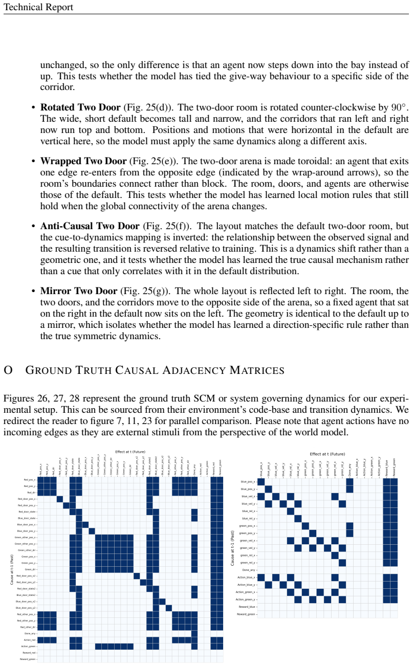
**Figure 26.** Figure 26: Ground truth causal adjacency matrices describing cause-effect relationship across time [PITH_FULL_IMAGE:figures/full_fig_p049_26.png]

**Figure 27.** Figure 27: Ground truth causal adjacency matrices describing cause-effect relationship across time [PITH_FULL_IMAGE:figures/full_fig_p050_27.png]

**Figure 28.** Figure 28: Ground truth causal adjacency matrices describing cause-effect relationship across time [PITH_FULL_IMAGE:figures/full_fig_p051_28.png]

**Figure 29.** Figure 29: Overview of the ∆variance testing framework. (a) Toy Environments: Controlled linearGaussian and two-agent navigation systems used to isolate dynamics. (b) Metric Computation: Pipeline normalizing model MSE by the variance floor σ 2 D to derive ∆variance. (c) Regimes…

**Figure 30.** Figure 30: Toy evaluation of density-based fault detection vs. the variance metric. (a) Two-agent [PITH_FULL_IMAGE:figures/full_fig_p057_30.png]

**Figure 31.** Figure 31: Causal Graph Perturbation Analysis. We evaluate the robustness of causal metrics against [PITH_FULL_IMAGE:figures/full_fig_p058_31.png]

**Figure 32.** Figure 32: Quantitative evaluation of the expert policy in various domains [PITH_FULL_IMAGE:figures/full_fig_p061_32.png]

**Figure 33.** Figure 33: Starting State of environments used to capture an adversarial agents intent. [PITH_FULL_IMAGE:figures/full_fig_p062_33.png]

**Figure 34.** Figure 34: Evaluation dataset configuration for multi-agent navigation scenarios involving two, [PITH_FULL_IMAGE:figures/full_fig_p063_34.png]

**Figure 35.** Figure 35: Recovered causal-graph error falls as interventional strength grows, across every environment, metric, and observation mode. Each of the six bordered panels reports one grapherror metric against the interventional strength σ of the training data, for the three coordi…

**Figure 36.** Figure 36: At high sample complexity, the intervention–recovery trend holds and the discovered graphs sharpen further. Recovered-graph error versus interventional strength σ for the giveway and two-door domains trained on the high-sample datasets (give-way ≈30k–120k transition…

**Figure 37.** Figure 37: This figure displays recovered causal graph structures for Give-Way and Two-Door en [PITH_FULL_IMAGE:figures/full_fig_p066_37.png]

**Figure 38.** Figure 38: Performance metrics for PCMCI and PC algorithm’s recovered graph in multi-agent [PITH_FULL_IMAGE:figures/full_fig_p067_38.png]

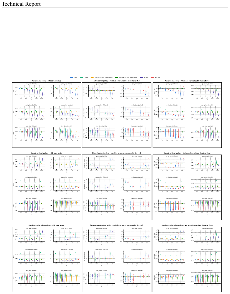
**Figure 39.** Figure 39: World-model one-step prediction error across the canonical three-environment sweep. Six architectures (AWM, C-VAE, FOCUS, BC-WM, ICWM, R-ICWM) trained on give way, navigation, and two door under full and partial observability, at intervention strengths σ ∈ {0.01, 0.25…

**Figure 40.** Figure 40: World-model one-step prediction error in the high-sample regime. Six architectures trained on enlarged datasets for give way (roughly 120k transitions) and two door (roughly 2M transitions) under full and partial observability, at intervention strengths σ ∈ {0.01, 0.…

**Figure 41.** Figure 41: Multi-agent world-model error with and without LIDAR. Six architectures trained on navigation with 2, 3, and 4 agents at intervention strengths σ ∈ {0, 0.25, 0.5}, evaluated on adversarial rollouts. Each metric (raw MSE, error relative to the same model at σ = 0.5, va…

**Figure 42.** Figure 42: Causal-mask ablation study (1,200 runs: 6 groups × 4 masks × 2 architectures × 5 intervention strengths × 5 seeds). (a) Relative error by mask for all six groups; row 1 full observability, row 2 partial or noisy observability. (b) Median error normalized to each grou…

**Figure 43.** Figure 43: Spine-and-cloud densities, two door (peak-height normalization: every density is rescaled to a maximum of one, so the width of each curve is the model’s uncertainty on that axis). Header: the green and red framed snapshots show the evaluated in-distribution and outof…

**Figure 44.** Figure 44: Spine-and-cloud densities, give way (peak-height normalization). Layout as in Figure 43, with two differences. Columns cross observability (full, noisy) with sample regime (normal, high), and actions are continuous: each optimal-action cell draws the agent’s 2-D velo…

**Figure 45.** Figure 45: Spine-and-cloud densities, navigation with 2 agents (peak-height normalization). Layout as in [PITH_FULL_IMAGE:figures/full_fig_p077_45.png]

**Figure 46.** Figure 46: Spine-and-cloud densities, navigation with 2 agents, no LIDAR (peak-height normalization). Same construction as [PITH_FULL_IMAGE:figures/full_fig_p078_46.png]

**Figure 47.** Figure 47: Spine-and-cloud densities, navigation with 3 agents, no LIDAR (peak-height normalization). Layout as in [PITH_FULL_IMAGE:figures/full_fig_p079_47.png]

**Figure 48.** Figure 48: Spine-and-cloud densities, navigation with 4 agents, no LIDAR (peak-height normalization). Layout as in [PITH_FULL_IMAGE:figures/full_fig_p080_48.png]

**Figure 49.** Figure 49: Quantifying per-axis uncertainty from the cloud widths (all 182 spine-cloud fits pooled; medians and IQRs throughout, since BC-WM’s off-distribution widths reach 105 normalized units and would dominate any mean). (a) Mean per-dimension cloud width per model on a fixe…

**Figure 50.** Figure 50: Per-axis uncertainty by environment with conditions overlaid. Rows: two door, give way, navigation, and navigation without LIDAR; note the per-row y scales and the different σ grids ({0.01, 0.5, 0.99} for the first two rows, {0, 0.25, 0.5} for the multi-agent rows). W…

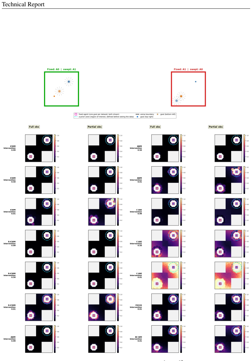
**Figure 51.** Figure 51: Spatial error density for two door, a discrete grid with one agent fixed next to the goal (blue) door. Each panel is a 13×6 error heatmap drawn over the room. Darker means lower error and brighter means higher error, on a colour scale shared across all panels. Magenta…

**Figure 52.** Figure 52: Spatial error density for give way, a continuous environment. It is a horizontal corridor with a give-way bay, the vertical notch, where one agent can pull aside and let the other pass. The fixed agent’s goal sits inside the corridor. The corridor and the bay are samp…

**Figure 53.** Figure 53: Spatial error density for navigation, a continuous [−1, 1]2 arena. The fixed agent sits on its goal and the moving agent is swept over a square region around it. The dashed white circle is the fixed agent’s LIDAR range, the only region where the two agents actually se…

**Figure 54.** Figure 54: Dynamics error density on Rotated Two Door. The header shows the two layouts side by side: the training room (left two panels, blue title border) and the same room turned 90◦ anticlockwise, so its left-right corridors now run top-bottom (right two panels, green/red ti…

**Figure 55.** Figure 55: Dynamics error density on Mirror Two Door: the room reflected about the vertical axis, so the closed goal (blue) door moves from the right side of the corridor to the left and the open (red) door moves the opposite way. Same row/column layout, overlays (magenta fixed …

**Figure 56.** Figure 56: Dynamics error density on Stretched Two Door: the room widened by one corridor column and stretched by four extra rows, so the agents now reach y-coordinates the training layout never visited. Unlike the rotation and the mirror, this shift adds genuinely unseen space …

**Figure 57.** Figure 57: Dynamics error density on Mirror Give Way: the give-way bay (the notch off the corridor where one agent waits for the other to pass) flipped from above the corridor to below it, while the corridor itself, the goals, the agent radius, and the action range are unchanged…

**Figure 58.** Figure 58: Dynamics error density on Wrap Two Door: the two-door layout is byte-identical to the training room (same walls, doors, legal cells, and grid size), but the transition function is changed so that each of the three rooms is a torus, and a forward step into a wall re-en…

**Figure 59.** Figure 59: Dynamics error density on Anti-Causal Two Door: the geometry is unchanged, but the joint state is placed off-manifold: the door states are swapped (blue open, red closed) and the pinned agent is moved to the red door, a sequentially impossible configuration since the …

**Figure 60.** Figure 60: Dynamics error density on Easy Give Way: exactly one feature’s geometry moves (the give-way notch is widened five-fold along x, passage 0.4 → 2.0), while the corridor, the goals, the agent radius, and the action range are all held fixed. The widened bay places the swe…

**Figure 61.** Figure 61: Give-way distortion by region, layout, model and intervention. Top: the three regions marked on the real geometry – Corridor Wall (grey), Corridor Connector (gold), Notch (red). Grid: rows are the three layouts (Source = unshifted reference, Easy, Mirror); column grou…

**Figure 62.** Figure 62: Recurrence helps where the training speed was low. (A) The three give-way regions. (B) Median training-time speed per region against intervention level (band: IQR; × marks a region never visited at that level). Wall is fastest, Notch slowest. (C) Median velocity-only …

**Figure 63.** Figure 63: Structural recovery versus counterfactual world-model error, pooled over 1,240 world [PITH_FULL_IMAGE:figures/full_fig_p102_63.png]

**Figure 64.** Figure 64: Does receiving a causal graph improve out-of-distribution prediction? Panel A compares [PITH_FULL_IMAGE:figures/full_fig_p102_64.png]

**Figure 65.** Figure 65: Intervention strength, not graph quality, drives counterfactual accuracy. Panel A: [PITH_FULL_IMAGE:figures/full_fig_p103_65.png]

**Figure 66.** Figure 66: Layout shift: the recovered graph buys no transferable physics. Frozen world models, [PITH_FULL_IMAGE:figures/full_fig_p103_66.png]

**Figure 67.** Figure 67: Where the causal mask pays off: partial observation and extrapolation on the Stretched [PITH_FULL_IMAGE:figures/full_fig_p104_67.png]

**Figure 68.** Figure 68: What decides when the mask helps: alignment and what moved, not the graph. The [PITH_FULL_IMAGE:figures/full_fig_p104_68.png]

**Figure 69.** Figure 69: Three controlled shifts, each isolating one factor the earlier layouts moved together. [PITH_FULL_IMAGE:figures/full_fig_p106_69.png]

**Figure 70.** Figure 70: The anti-causal firewall is intervention-learned, model-specific, and shift-specific. [PITH_FULL_IMAGE:figures/full_fig_p106_70.png]

Discussion (0). Sign in to comment.

Reference graph

Works this paper leans on

13 extracted references · 5 linked inside Pith

[1]

We assumeu env ⊥ ⊥uintent

Environmental Stochasticity (u env): Represents irreducible noise (e.g., friction, jitter, weather conditions). We assumeu env ⊥ ⊥uintent. This term dictates predictive vari- ance (kernel thickness or uncertainty in the model’s output), which we do not explicitly 21 Technical Report deconfound. We assumeu env is captured by dataset variance and offer no s...
[2]

Daniel Kumor, Junzhe Zhang, and Elias Bareinboim

URLhttps://arxiv.org/abs/1911.12247. Daniel Kumor, Junzhe Zhang, and Elias Bareinboim. Sequential causal imitation learning with unobserved confounders, 2022. URLhttps://arxiv.org/abs/2208.06276. Yann LeCun et al. A path towards autonomous machine intelligence version 0.9. 2, 2022-06-27. Open Review, 62(1):1–62, 2022. Kenneth Li, Aspen K. Hopkins, David B...

arXiv 1911
[3]

Open Blue Door Two Door Environment
[6]

Agents Reach Goal Give-way Environment Figure 24: Environments used for empirical experiments. L STATEREPRESENTATION OFDIFFERENT ENVIRONMENTS L.1 TWO-DOORCOORDINATION •Variables: LetP i = [xi, yi, di]be the state of agenti∈ {R, G}andDj = [sj, xj, yj]be the state of doorj∈ {Red, Blue}, wheresj ∈ {0,1}denotes door status. •Full Observability (MDP): The stat...
[8]

fair experiment

Strategic Confounding (u i intent): Represents unobserved coordination signals that correlate withs t in expert data, creating backdoor paths (s t ←u i intent →a i t →s t+1) that cause associative models to mistake agent choice for physical law. We address this by leveraging policy variance (soft interventions) to satisfy the Sequential Backdoor Condition...

2018
[11]

Agents Reach Goal Navigation Environment
[12]

Agents Avoid Collation
[14]

hardness

MiniGrid actions representintent-based navi- gation, where state transitions are deterministic and independent of force magnitude. This difference fundamentally changes the learning objective from navigating a continuous en- ergy manifold to optimizing a sequence of symbolic decision-making steps. N SHIFTED ENVIRONMENTS (a) Stretched Two Door Environment ...

2017

Show all 13 references

[1988]

Christian Reiser

URLhttps://proceedings.neurips.cc/paper_files/paper/1988/ file/812b4ba287f5ee0bc9d43bbf5bbe87fb-Paper.pdf. Christian Reiser. Causal discovery for time series with latent confounders, 2022. URLhttps: //arxiv.org/abs/2209.03427. 13 Technical Report Thomas Richardson and Peter Sp...

1988 arXiv
[1990]

ISBN 0444892648

Elsevier Science Inc. ISBN 0444892648. John V on Neumann and Oskar Morgenstern.Theory of Games and Economic Behavior. Princeton University Press, Princeton, NJ, 1944. Tsachy Weissman, Erik Ordentlich, Gadiel Seroussi, Sergio Verd ´u, and Marcelo J. Weinberger. Inequalities for...

1944 arXiv
[2020]

Mahmoud Assran, Quentin Duval, Ishan Misra, Piotr Bojanowski, Pascal Vincent, Michael Rabbat, Yann LeCun, and Nicolas Ballas

URLhttps://arxiv.org/abs/1907.02893. Mahmoud Assran, Quentin Duval, Ishan Misra, Piotr Bojanowski, Pascal Vincent, Michael Rabbat, Yann LeCun, and Nicolas Ballas. Self-supervised learning from images with a joint-embedding predictive architecture, 2023. URLhttps://arxiv.org/ab...

1907 arXiv
[2024]

Ryan Lowe, Yi Wu, Aviv Tamar, Jean Harb, Pieter Abbeel, and Igor Mordatch

URLhttps://arxiv.org/abs/2210.13382. Ryan Lowe, Yi Wu, Aviv Tamar, Jean Harb, Pieter Abbeel, and Igor Mordatch. Multi-agent actor- critic for mixed cooperative-competitive environments, 2020. URLhttps://arxiv.org/ abs/1706.02275. 12 Technical Report Yuzhe Lu, Yilong Qin, Runti...

2020 arXiv
[9227]

URLhttps://doi.org/10.1109/TNN.2008

doi: 10.1109/TNN.2008.2005605. URLhttps://doi.org/10.1109/TNN.2008. 2005605. Matthew Schlegel, Wesley Chung, Daniel Graves, Jian Qian, and Martha White. Importance resam- pling for off-policy prediction, 2019. URLhttps://arxiv.org/abs/1906.04328. Bernhard Sch¨olkopf and Alexan...

2008

Pith tools

Reviewed August 1, 2026 · model on record in the stance chip above.

[1] [1]

We assumeu env ⊥ ⊥uintent

Environmental Stochasticity (u env): Represents irreducible noise (e.g., friction, jitter, weather conditions). We assumeu env ⊥ ⊥uintent. This term dictates predictive vari- ance (kernel thickness or uncertainty in the model’s output), which we do not explicitly 21 Technical Report deconfound. We assumeu env is captured by dataset variance and offer no s...

[2] [2]

Daniel Kumor, Junzhe Zhang, and Elias Bareinboim

URLhttps://arxiv.org/abs/1911.12247. Daniel Kumor, Junzhe Zhang, and Elias Bareinboim. Sequential causal imitation learning with unobserved confounders, 2022. URLhttps://arxiv.org/abs/2208.06276. Yann LeCun et al. A path towards autonomous machine intelligence version 0.9. 2, 2022-06-27. Open Review, 62(1):1–62, 2022. Kenneth Li, Aspen K. Hopkins, David B...

arXiv 1911

[3] [3]

Open Blue Door Two Door Environment

[4] [6]

Agents Reach Goal Give-way Environment Figure 24: Environments used for empirical experiments. L STATEREPRESENTATION OFDIFFERENT ENVIRONMENTS L.1 TWO-DOORCOORDINATION •Variables: LetP i = [xi, yi, di]be the state of agenti∈ {R, G}andDj = [sj, xj, yj]be the state of doorj∈ {Red, Blue}, wheresj ∈ {0,1}denotes door status. •Full Observability (MDP): The stat...

[5] [8]

fair experiment

Strategic Confounding (u i intent): Represents unobserved coordination signals that correlate withs t in expert data, creating backdoor paths (s t ←u i intent →a i t →s t+1) that cause associative models to mistake agent choice for physical law. We address this by leveraging policy variance (soft interventions) to satisfy the Sequential Backdoor Condition...

2018

[6] [11]

Agents Reach Goal Navigation Environment

[7] [12]

Agents Avoid Collation

[8] [14]

hardness

MiniGrid actions representintent-based navi- gation, where state transitions are deterministic and independent of force magnitude. This difference fundamentally changes the learning objective from navigating a continuous en- ergy manifold to optimizing a sequence of symbolic decision-making steps. N SHIFTED ENVIRONMENTS (a) Stretched Two Door Environment ...

2017