REVIEW 4 major objections 6 minor 24 references
Learning Energy-Based Generative Models via Potential Flow: A Variational Principle Approach to Probability Density Homotopy Matching
T0 review · 4 major / 6 minor · reviewed 2026-08-16 · deepseek-v4-flash
Pith's one-line read VPFB trains an energy-based model by matching a potential-flow density path to the data, replacing MCMC negative sampling with a variational Poisson-equation loss.
desk verdict A promising MCMC-free EBM training scheme that earns referee time, but the central theoretical claim overreaches: Prop. 3 assumes the homotopy equality it needs to prove, and the implemented loss differs from the proved one. read the letter →
The pith
A machine-rendered reading of the paper's core claim, the machinery that carries it, and where it could break.
The reading
What carries the argument
The argument is carried by three linked objects. First, the conditional density homotopy $\rho(x|\bar{x},t) \propto \exp(\alpha(t)\log q(x) + \beta(t)\log p(\bar{x}|x))$, which the paper shows is a Gaussian perturbation kernel $\mathcal{N}(\mu(t)\bar{x}, \sigma(t)^2 I)$ interpolating between a Gaussian prior and the data-conditioned posterior; marginalizing it over data defines the target path $\bar{\rho}(x,t)$. Second, the density-weighted Poisson equation $\nabla\cdot(\bar{\rho}\nabla\Phi) = \frac12\,\mathbb{E}_{p_{\text{data}}}[\rho(\gamma-\bar{\gamma})]$, which encodes equality of the flow-driven density and the target homotopy, with innovation term $\gamma = (\dot{\alpha}/\omega^2)\|x\|^2 + (\dot{\beta}/\nu^2)\|x-\bar{x}\|^2$ centered at its conditional mean $\bar{\gamma}$. Third, the Deep Ritz loss $L(\Phi,t) = \operatorname{Cov}_{\rho p_{\text{data}}}[\Phi,\gamma] + \mathbb{E}_{\bar{\rho}}[\|\nabla\Phi\|^2]$, whose first-order optimality condition reproduces the weak form of the Poisson equation; a Poincar\'e-type spectral gap is invoked to guarantee a unique minimizer. The Boltzmann energy identity $\Phi_B = (4\Phi_\infty + f_\infty\|x\|^2)/g_\infty^2$ then connects the steady-state potential to the EBM likelihood, and the implemented training loss adds a cosine alignment term between $\nabla\Phi$ and the flow-matching conditional vector field plus a quasi-static penalty on $\partial\Phi/\partial t$.
What would settle it
On a low-dimensional target with a known density, such as a Gaussian mixture in two dimensions, train VPFB and then estimate the true density of the ODE-transported particles at several intermediate times by histogram or kernel binning; if the KL divergence between that measured flow density and the analytic marginal homotopy $\bar{\rho}(x,t)$ does not decrease toward zero as the Deep Ritz loss is minimized, the equivalence claimed in Proposition 3 is contradicted. A second, cheaper check: evaluate the residual of the density-weighted Poisson equation using the learned $\Phi$ and Monte Carlo estimates of the innovation expectation; a nonzero residual at the converged loss minimum would show the variational loss is not solving the PDE it claims to solve.
Extended reading notes
Core claim
VPFB's central claim is that training an energy-based generative model reduces to a variational-principle problem: rather than sampling negative examples with MCMC, one learns a potential $\Phi(x,t)$ whose gradient field transports a Gaussian prior along a density path that matches a prescribed homotopy to the data. The paper proves (Propositions 3 and 6) that solving the density-weighted Poisson equation $\nabla\cdot(\bar{\rho}\nabla\Phi) = \frac12\,\mathbb{E}[\rho(\gamma-\bar{\gamma})]$ is equivalent to minimizing the KL divergence between the flow-driven density and the target marginal homotopy, and that this is in turn equivalent to minimizing a Deep Ritz loss consisting of a covariance between the potential and the innovation $\gamma$ plus the expected squared gradient norm. At stationarity (Proposition 5), the same potential parameterizes a Boltzmann energy $\Phi_B = (4\Phi_\infty + f_\infty\|x\|^2)/g_\infty^2$, so the trained network is simultaneously a sampler and an energy surface for OOD detection. Training freezes the flow near the terminal time and treats the truncated marginal as the data distribution, making the Boltzmann form hold by construction rather than by demonstrated convergence.
Load-bearing premise
The load-bearing premise is that the flow-driven density already equals the target marginal homotopy: the proof of Proposition 3 derives the density-weighted Poisson equation from the KL objective only after assuming $\rho_\Phi(x,t) \equiv \bar{\rho}(x,t)$, the very equality the training is supposed to produce, and the stationarity claim similarly treats the truncated marginal at $t_{\max}$ as the data distribution by construction.
Editorial extensions
If this is right
- EBM training reduces to a gradient-descent objective, a covariance loss plus gradient-norm penalty, with no MCMC negative sampling, so the main cost and instability of contrastive divergence disappears.
- The trained potential is an explicit Boltzmann energy: the same network generates samples by ODE or SGLD and assigns energies that separate in-distribution from out-of-distribution inputs, as the paper's AUROC experiments demonstrate.
- Because the training path is the optimal-transport flow-matching schedule, particle trajectories are nearly straight, so deterministic ODE sampling reaches competitive FID (6.72 on CIFAR-10 for the time-varying model) at a fraction of the training cost of the MCMC-based EBM baselines reported in the paper.
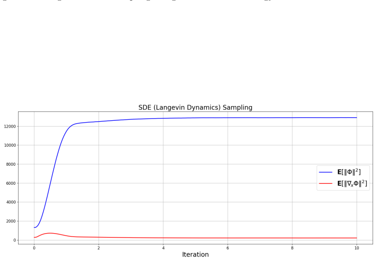
- The MCMC-free promise applies to training: at inference, long-run deterministic ODE sampling drifts into visual artifacts in high dimensions, and the paper finds that stochastic SGLD sampling from the learned Boltzmann energy is what reaches the steady-state equilibrium.
- Compositional generation becomes energy averaging: conditioning on a combination of attributes is approximated by averaging conditional potentials, which the paper demonstrates on CelebA attribute pairs.
Reading between the lines
- If Proposition 3's equivalence is as general as stated, the same variational principle should transfer to other perturbation kernels, such as heat-equation blurring or general linear corruptions, by recomputing the innovation term; the paper points to Neumann-boundary blurring kernels as future work, but the variational structure suggests the swap is mechanical.
- The Boltzmann interpretation stands or falls with how close the truncated marginal $\bar{\rho}(x,t_{\max})$ is to the data; the paper's AUROC scores vary noticeably across OOD datasets, suggesting the energy's discriminative strength is dataset-dependent in a way the proof does not quantify.
- The added cosine-alignment and quasi-static terms in the implemented loss go beyond the variational derivation, so the learned $\Phi$ is a Boltzmann energy only up to how strongly these extra terms perturb the minimizer; an ablation at fixed FID that isolates their effect on the energy's equilibrium behavior would clarify their role.
- Because the covariance loss ties the energy magnitude to the residual of a Gaussian fit, the framework may be sensitive to the Gaussianity of the conditional path; extending the SDE formulation to non-Gaussian or learned priors, which the paper flags as a limitation, would test whether the energy-based interpretation survives beyond unimodal Gaussian transport.
Signed reviews
Editorial analysis
A structured set of objections, weighed in public.
Referee Report
Summary. The paper proposes Variational Potential Flow Bayes (VPFB), a framework for training energy-based generative models without contrastive divergence or auxiliary networks. The method parameterizes a potential flow Phi(x,t) and aims to match the flow-driven density homotopy to a data-recovery marginal homotopy built from Gaussian perturbation kernels. The authors derive a density-weighted Poisson equation (Eq. 14) as a stationarity condition, reformulate it as a Deep Ritz / covariance variational loss (Eq. 22), and claim that at stationarity the learned potential equals a Boltzmann energy (Eq. 20) usable for generation, interpolation, compositional generation, and OOD detection. Experiments on 2D synthetic densities, CIFAR-10, and CelebA report competitive FID and AUROC scores, with additional ablations and efficiency comparisons in the appendices.
Significance. If the theoretical claims were fully established, VPFB would be a significant contribution: it offers a sampling-free training objective for explicit EBMs, an interpretable energy landscape, OOD detection as a by-product, and a clear connection between potential flow and diffusion/flow-matching theory. The use of the Deep Ritz method for a density-weighted Poisson equation in generative modeling is novel and interesting. The paper is also unusually honest about its limitations, including long-run ODE divergence, the need for SGLD at inference, and the trade-off between Boltzmann stationarity and sample quality. However, the central theoretical bridge is currently not proven: Proposition 3's proof assumes the homotopy equality it is meant to establish, stationarity is enforced by construction in Section 3.5, and the implemented loss (25) differs from the analyzed loss (22). These gaps mean the paper's headline claims outrun the supporting theory, and the empirical results lack repeated-run statistics. The idea is promising and the empirical core may be salvageable, but substantial revision is required.
major comments (4)
- [Section 3.2 / Appendix C.3, Eq. (61)] Proposition 3's equivalence claim between solving the density-weighted Poisson equation (14) and minimizing the KL divergence D_KL[rho_Phi || rho_bar] is not established. In the proof of Proposition 3, the first variation of the one-step KL is computed for a general rho_Phi, but equation (61) then substitutes rho_Phi(x,t) ≡ rho_bar(x,t) before deriving the Poisson equation. Consequently, equation (14) is a local condition that preserves homotopy matching provided the flow density is already on the target marginal; the proof does not show that minimizing the loss in (22) contracts the KL when rho_Phi differs from rho_bar, which is precisely the situation during training of a finite-capacity network. This is load-bearing because the paper uses Proposition 3 to claim that the variational loss minimizes KL divergence between homotopies (see Section 3.4 and the remark following Proposition 6). The authors should either prove a contraction or bound for the KL under the proposed loss, or explicitly restate Proposition 3 as a preservation property and temper the framing accordingly.
- [Section 3.5, Eq. (20)] The stationary Boltzmann equilibrium is imposed by fiat: the text sets p_infinity(x) = rho_bar(x, t >= t_max) ≈ p_data(x) and then equates this to the Boltzmann distribution. As written, 'the stationary Boltzmann distribution approximates the true data likelihood by design', so the learned energy approximates the data by construction rather than by convergence of the learning procedure. Proposition 5's conclusion is therefore conditional on an assumption that is not derived from the flow-matching dynamics and is not empirically verified. This is load-bearing for the claim that VPFB learns an explicit EBM whose energy is a valid OOD score. The authors should provide a quantitative assessment of the discrepancy between rho_bar(x, t_max) and p_data (for example, an FID or likelihood evaluation of the marginal at the cutoff), or clearly label the stationarity enforcement as an additional modeling assumption separate from the theoretical claims.
- [Section 3.4-3.5, Eqs. (22) and (25)] The implemented loss (25) differs from the theoretically analyzed loss (22) by the cosine alignment term, the Poincare regularization η||Phi||^2, the time-derivative penalty, and the weighting w(t). No theorem connects this full implemented loss to the weak formulation (21) or to the KL minimization claim of Proposition 3. The cosine term, in particular, changes the scale-invariance properties of the objective, and the Poincare penalty changes the minimizer of the variational problem. The ablation study in Table 3 shows these terms are empirically important, but the theory section only covers loss (22). As a result, the claim that the actual training procedure optimizes the proposed KL/Deep Ritz objective is unsupported. The authors should either extend the theoretical analysis to the full loss (25) or explicitly present (25) as an empirically motivated modification whose relationship to (22) is to be established.
- [Tables 1 and 2] The paper reports single FID and AUROC values without standard deviations or multiple seeds. FID estimates are known to be noisy, and several reported margins over competitors are small (for example, VPFB's FID 6.72 versus Flow Matching's 6.35, or AUROC 0.78 versus CDRL's 0.75 on CIFAR-10). The checkpoint selection rule (lowest FID on a validation subset, per Appendix D.5) further biases the reported numbers. Since the empirical claims of competitiveness are a major part of the paper's contribution, the authors should provide means and standard errors over at least three independent training runs, or clearly state that the results are single-run and interpret them as preliminary without strong comparative statements.
minor comments (6)
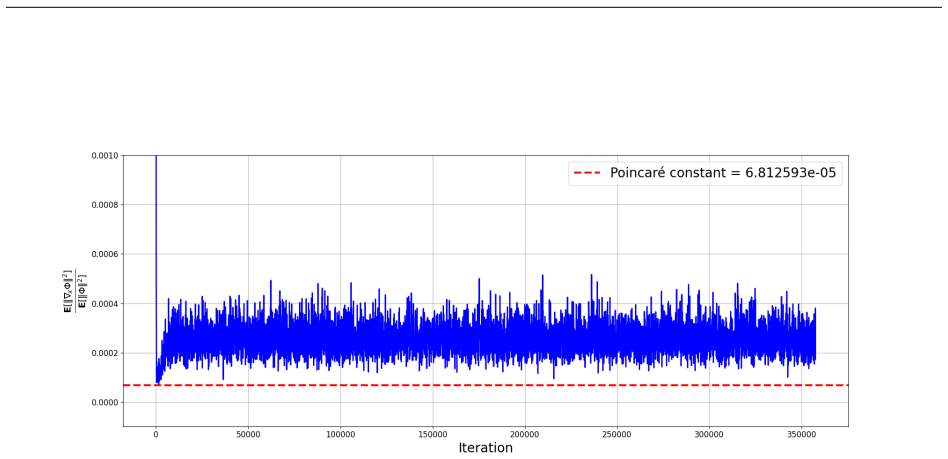
- [Eq. (25)] The gradient-norm term in Eq. (25) writes ∇_{(x,t)}Phi, which appears to be a typo for ∇_x Phi; in addition, the time-derivative penalty mentioned in the text is not explicitly displayed in the equation.
- [Section 3.2 / Appendix C.3] The notation for the Sobolev space is inconsistent: Proposition 3 states Phi in H^1_0(Ω,p) while the text earlier defines H^n_0; please harmonize the notation throughout.
- [Eq. (16)] The diffusion coefficient formula g(t) = -√(2σ(t)(σ̇(t)+f(t)σ(t))) carries a minus sign outside the square root; since g is conventionally positive, please verify the sign convention and define the square-root branch explicitly.
- [Figure 10] The caption should clarify that the plotted ratio is measured while training without the Poincare regularization, whereas the final models include the Poincare penalty; as written, the figure may be misinterpreted as validating the final loss.
- [Table 1] The column header 'Other Likelihood-based Models' includes GAN-based models such as SN-GAN and BigGAN, which are not likelihood-based; please reorganize the table or adjust the caption to avoid confusion.
- [Appendix D.2 and D.3] The training setup states a terminal time of tend = 1, while Appendix D.3 states that best ODE sampling results use tend = 1.575; please clarify the distinction between training and sampling time horizons.
Circularity Check
Proposition 3's proof assumes the homotopy equality it claims to derive, and Section 3.5 imposes the Boltzmann stationary state by defining p∞(x) = ρ̄(x,t≥tmax) ≈ p_data.
-
self definitional
[Appendix C.3, after Eq. (61) in the proof of Proposition 3]
"where we have assumed that ρΦ(x,t)≡¯ρ(x,t) holds and have used the following identities:"
Proposition 3 is the load-bearing claim that solving the density-weighted Poisson equation (14) is equivalent to minimizing DKL[ρΦ∥ρ̄], and Proposition 6 then links loss (22) to that equation. In the proof, after deriving the first variation for a general trial direction, the text substitutes ρΦ(x,t)≡ρ̄(x,t) before obtaining the PDE. With the base case ρΦ(x,0)=ρ̄(x,0), this gives only a local preservation result: if the flow density is already on the target homotopy, the constructed velocity keeps it there. It does not show that the loss contracts the KL divergence when ρΦ differs from ρ̄, which is precisely the finite-capacity network / SGD situation.
-
fitted input called prediction
[Section 3.5, Training Implementation]
"we explicitly enforce stationarity in our training implementation, by imposing a steady-state equilibrium p∞(x) = ¯ρ(x,t≥tmax) ... This steady-state equilibrium p∞(x)≡pB(x) thus corresponds to the stationary Boltzmann distribution ... Given that a steady-state equilibrium is enforced via p∞(x) = ¯ρ(x,t≥tmax)≈pdata(¯x), the stationary Boltzmann distribution approximates the true data likelihood by design."
The paper's advertised connection between the learned potential and the Boltzmann energy (20) rests on the marginal homotopy reaching a stationary equilibrium. The text concedes that ρ̄ is not guaranteed to reach equilibrium within the flow's finite time window, and then fixes the gap by declaring p∞(x) = ρ̄(x,t≥tmax) ≈ p_data. Since the stationary density is set equal to the schedule's terminal marginal and asserted to approximate p_data by design, the Boltzmann energy Φ_B is tied to the chosen schedule by construction rather than being a converged prediction of the homotopy-matching loss. The central claim that VPFB learns a stationary Boltzmann energy is therefore partly an enforced definition, not an independently derived consequence.
full rationale
The paper does contain a genuinely meaningful independent ingredient: the Deep Ritz / covariance-plus-gradient loss (22) is a legitimate variational form for the density-weighted Poisson equation, and the experiments are benchmarked against external methods rather than only against the authors' own outputs. No load-bearing self-citation chain or imported uniqueness theorem from the same authors appears. However, the theoretical bridge from the KL objective to the implemented loss is broken by two explicit insertions. In the proof of Proposition 3, the equality ρΦ≡ρ̄ is assumed at Eq. (61) before the Poisson equation is derived, so the proof establishes only preservation of an already-assumed matching, not convergence of the KL objective from a mismatched density. In Section 3.5, stationarity is imposed by fiat: p∞(x) is defined as ρ̄(x,t≥tmax) and then taken to approximate p_data, making the Boltzmann energy approximate the data by construction. Because these two steps are located on the central derivation path from the variational principle to the claimed EBM/Boltzmann result, the core theoretical claim is partially circular, even though the empirical evaluation and the Deep Ritz formulation retain independent value. A score of 7 reflects this partial but central circularity; it is not a case of mere incidental self-citation.
Assumptions & free parameters
free parameters (6)
- OT-FM mean schedule mu(t) =
t
- OT-FM standard deviation schedule sigma(t) =
1 - t
- Cutoff time t_max =
1 - 1e-5
- Decay exponent kappa =
1.5
- Poincare spectral gap constant eta =
1e-4 (fine-tuned)
- SGLD temperature lambda =
0.35
assumptions (6)
- standard math Flow density evolves by the continuity equation (12).
- domain assumption The prior is a unimodal Gaussian q(x) = N(0, omega^2 I).
- domain assumption The marginal density rho_bar vanishes on the boundary of the domain.
- domain assumption The Poincare inequality holds with a positive constant eta.
- ad hoc to paper Stationary equilibrium can be enforced by setting p_infinity(x) = rho_bar(x, t >= t_max) approximately p_data.
- ad hoc to paper The flow-driven density equals the target marginal homotopy inside the proof of Proposition 3.
Cite this review
Pith. "Pith review of Learning Energy-Based Generative Models via Potential Flow: A Variational Principle Approach to Probability Density Homotopy Matching." pith.science (2026). https://pith.science/paper/JIAAJB5L
@misc{pith2026250416262,
  author       = {Pith},
  title        = {Pith review of: Learning Energy-Based Generative Models via Potential Flow: A Variational Principle Approach to Probability Density Homotopy Matching},
  year         = {2026},
  howpublished = {\url{https://pith.science/paper/JIAAJB5L}},
  note         = {Machine review of arXiv:2504.16262}
}
read the original abstract
Energy-based models (EBMs) are a powerful class of probabilistic generative models due to their flexibility and interpretability. However, relationships between potential flows and explicit EBMs remain underexplored, while contrastive divergence training via implicit Markov chain Monte Carlo (MCMC) sampling is often unstable and expensive in high-dimensional settings. In this paper, we propose Variational Potential Flow Bayes (VPFB), a new energy-based generative framework that eliminates the need for implicit MCMC sampling and does not rely on auxiliary networks or cooperative training. VPFB learns an energy-parameterized potential flow by constructing a flow-driven density homotopy that is matched to the data distribution through a variational loss minimizing the Kullback-Leibler divergence between the flow-driven and marginal homotopies. This principled formulation enables robust and efficient generative modeling while preserving the interpretability of EBMs. Experimental results on image generation, interpolation, out-of-distribution detection, and compositional generation confirm the effectiveness of VPFB, showing that our method performs competitively with existing approaches in terms of sample quality and versatility across diverse generative modeling tasks.
Figures


Figures from the paper (19 more)









Reference graph
Works this paper leans on
-
[5]
This process helps smoothout sharplocal minimaand mitigatesoverfittingto high-densityareas
B.2 Incorporating Langevin Dynamics for Boltzmann-Convergent Sampling Conventional EBM training often relies on convergent (long-run) MCMC sampling to thoroughly explore the data space and assign appropriate energy values across the landscape, particularly in low-density regions. This process helps smoothout sharplocal minimaand mitigatesoverfittingto hig...
work page 2019
-
[7]
Johannes Müller and Marius Zeinhofer. Deep ritz revisited. InICLR 2020 Workshop on Integration of Deep Neural Models and Differential Equations,
work page 2020
-
[8]
U-net: Convolutional networks for biomedical image segmentation
Olaf Ronneberger, Philipp Fischer, and Thomas Brox. U-net: Convolutional networks for biomedical image segmentation. InMedical Image Computing and Computer-Assisted Intervention – MICCAI 2015, pp. 234–241, Cham,
work page 2015
-
[9]
Springer International Publishing. Tim Salimans and Jonathan Ho. Should EBMs model the energy or the score? InEnergy Based Models Workshop - ICLR 2021,
work page 2021
-
[12]
Sergey Zagoruyko and Nikos Komodakis. Wide Residual Networks. InBritish Machine Vision Conference 2016, York, France, January
work page 2016
-
[13]
doi: 10.48550/arXiv.1605.07146
British Machine Vision Association. doi: 10.48550/arXiv.1605.07146. Yang Zhao, Jianwen Xie, and Ping Li. Learning energy-based generative models via coarse-to-fine expanding and sampling. InInternational Conference on Learning Representations,
-
[16]
(2021b), (2) an energy model parameterized by the NCSN++ architecture from Song et al
utilizes a multi-model architecture comprising three distinct components: (1) a generator model parameterized by the modified U-Net archi- tecture of Xiao et al. (2021b), (2) an energy model parameterized by the NCSN++ architecture from Song et al. (2021), and (3) a CNN-based encoder. This multi-component architecture enables specialized modules to collab...
work page 2021
-
[17]
Substituting this result along withu(x) =∇xΦ(x)into (64), we arrive at the following PDE: ∇x· ( ¯ρ(x,t)∇xΦ(x) ) = 1 2 Epdata(¯x) [ ρ(x|¯x,t) ( γ(x,¯x,t)−¯γ(x,¯x,t) )] (67) Therefore, assuming that the base caseρ0(x)≡¯ρ0(x)holds and that a solution to (67) exists at everyt, the proposition follows by the principle of induction. C.4 Proof of Proposition 4 T...
work page 2021
Show all 24 references
-
[18]
C.5 Proof of Proposition 5 Proof.Based on the result of Proposition 4 and using (12), we can express the homotopy matching problem ∂ρΦ(x,t) dt = ∂¯ρ(x,t) dt (74) equivalently as ∇x· ( ρΦ∇xΦ(x,t) ) =∇ x· ( ρΦ ( −f(t)x(t) + 1 2g(t)2∇x log ¯ρ(x,t) )) (75) Given that this matching...
2021
-
[19]
The optimal solutionΦof the functional (84) is given by the first-order optimality condition: I(Φ,Ψ) = d dϵL(Φ(x) +ϵΨ(x),t) ⏐⏐⏐⏐ ϵ=0 = 0(85) which must hold for all trial functionΨ
For an unnormal- ized solutionΦ(x), we can always obtain a normalization by subtracting its mean. The optimal solutionΦof the functional (84) is given by the first-order optimality condition: I(Φ,Ψ) = d dϵL(Φ(x) +ϵΨ(x),t) ⏐⏐⏐⏐ ϵ=0 = 0(85) which must hold for all trial function...
2015
-
[20]
For WideResNet, we include a spectral regularization loss during model training to penalize the spectral norm of the convolutional layer
and the U-Net (Ronneberger et al., 2015), respectively. For WideResNet, we include a spectral regularization loss during model training to penalize the spectral norm of the convolutional layer. Also, we apply weight normalization with data-dependent initialization (Salimans & Kingma,
2015
-
[21]
Our WideResNet architecture adopts the model hyperparameters reported by Xiao et al
on the convolutional layers to further regularize the model’s output. Our WideResNet architecture adopts the model hyperparameters reported by Xiao et al. (2021a). For U-Net, we remove the final scale-by-sigma operation (Kim et al., 2021; Song et al.,
2021
-
[23]
We find that Lamb performs better than Adam over large learning rates
and a learning rate of10−3 for all the experiments. We find that Lamb performs better than Adam over large learning rates. We use a batch size of 128 and 64 for training CIFAR-10 and CelebA, respectively. For all experiments, we set a cutoff time oftmax = 1−10 −5, a terminal t...
2022
-
[24]
CIFAR-10 consists of50,000training images and10,000test images at a resolution of32×32
datasets. CIFAR-10 consists of50,000training images and10,000test images at a resolution of32×32. The CelebA dataset contains202,599face images, with162,770used for training and19,962for testing. Each image is first cropped to178×178before being resized to64×64. During resizin...
2017
-
[1980]
doi: https://doi.org/10.1016/0771-050X(80) 90013-3
ISSN 0377-0427. doi: https://doi.org/10.1016/0771-050X(80) 90013-3. Yilun Du and Igor Mordatch. Implicit generation and modeling with energy based models. InAdvances in Neural Information Processing Systems, volume 32,
-
[2007]
Yuntian Deng, Anton Bakhtin, Myle Ott, Arthur Szlam, and Marc’Aurelio Ranzato
doi: 10.1117/12.725684. Yuntian Deng, Anton Bakhtin, Myle Ott, Arthur Szlam, and Marc’Aurelio Ranzato. Residual energy-based models for text generation. InInternational Conference on Learning Representations,
-
[2015]
Knowledge distillation in iterative generative models for improved sampling speed.arXiv preprint arXiv:2101.02388,
Eric Luhman, Troy Luhman, and Troy Luhman. Knowledge distillation in iterative generative models for improved sampling speed.arXiv preprint arXiv:2101.02388,
-
[2016]
Pixelcnn++: Improving the pixelcnn with discretized logistic mixture likelihood and other modifications.arXiv preprint arXiv:1701.05517,
Tim Salimans, Andrej Karpathy, Xi Chen, and Diederik P Kingma. Pixelcnn++: Improving the pixelcnn with discretized logistic mixture likelihood and other modifications.arXiv preprint arXiv:1701.05517,
-
[2018]
Reconstruction of pairwise interactions using energy-based models*
Christoph Feinauer and Carlo Lucibello. Reconstruction of pairwise interactions using energy-based models*. Journal of Statistical Mechanics: Theory and Experiment, 2021(12):124007,
2021
-
[2020]
Generative pointnet: Deep energy- based learning on unordered point sets for 3d generation, reconstruction and classification
Jianwen Xie, Yifei Xu, Zilong Zheng, Song-Chun Zhu, and Ying Nian Wu. Generative pointnet: Deep energy- based learning on unordered point sets for 3d generation, reconstruction and classification. InProceedings of the IEEE/CVF Conference on Computer Vision and Pattern Recognit...
-
[2021]
Our U-Net architecture adopts the hyperparameters used by Lipman et al
and replace it with the Euclidean norm 1 2∥x−f θ(x)∥2 computed between the inputx(t)and the output of the U-Netf θ(x). Our U-Net architecture adopts the hyperparameters used by Lipman et al. (2023). In both the WideResNet and U-Net models, we replace LeakyReLU activations with...
2023
-
[2022]
Soft truncation: A universal training technique of score-based diffusion model for high precision score estimation.arXiv preprint arXiv:2106.05527,
Dongjun Kim, Seungjae Shin, Kyungwoo Song, Wanmo Kang, and Il-Chul Moon. Soft truncation: A universal training technique of score-based diffusion model for high precision score estimation.arXiv preprint arXiv:2106.05527,
-
[2023]
GraphEBM: Molecular graph generation with energy-based models
Meng Liu, Keqiang Yan, Bora Oztekin, and Shuiwang Ji. GraphEBM: Molecular graph generation with energy-based models. InEnergy Based Models Workshop - ICLR 2021,
2021
-
[2024]
19 A Additional Results In this section, we present additional experiments that further validate the effectiveness and efficiency of the proposed VPFB framework. We first conduct an ablation study to evaluate the contribution of key loss components and architectural choices, d...
2023
Reviewed August 16, 2026 · model on record in the stance chip above.
Discussion (0). Continue with ORCID to comment.