REVIEW 3 major objections 5 minor 187 references
In physical QCD, the Chiral Separation Effect conductivity is suppressed in the hadronic phase and jumps sharply through the QCD crossover to the free-fermion value, while the Chiral Magnetic Effect conductivity vanishes in thermal equilibr
Reviewed by Pith at T0; open to challenge. T0 means a machine referee read the full paper against a public rubric. the ladder, T0–T4 →
T0 review · deepseek-v4-flash
2026-08-04 23:11 UTC pith:JS3NL3TJ
load-bearing objection First non-perturbative CSE conductivity at the physical point plus a convincing conserved-current explanation for the vanishing equilibrium CME; the rooting caveat is real but honestly disclosed. the 3 major comments →
Lattice QCD Study of Anomalous Transport Phenomena in Strongly Interacting Matter
The pith
A machine-rendered reading of the paper's core claim, the machinery that carries it, and where it could break.
Core claim
Central claim: in physical QCD with 2+1 flavors, the CSE conductivity (the axial-current response to a baryon chemical potential at vanishing chemical potential) is severely suppressed at low temperature, rises sharply through the QCD crossover, and reaches the massless free-fermion value 1/(2π²) at high temperature — this is the first non-perturbative anomalous-transport conductivity in physical QCD. For the CME, the claim is that the conductivity vanishes in global thermal equilibrium, both for free fermions and in QCD, whenever the current is the conserved vector current, and that previous non-vanishing equilibrium CME results are artifacts of non-conserved local currents. The paper furth
What carries the argument
Bloch's theorem (no globally conserved current flows in the equilibrium ground state in the thermodynamic limit) is the organizing principle: it forbids a global equilibrium CME but not the CSE, whose axial current is not conserved. The technical carrier is the lattice definition of the currents: the conserved, point-split vector current and the anomalous axial current, contrasted with the non-conserved local current responsible for spurious CME signals. CSE and CME coefficients are defined as Taylor coefficients at zero chemical potential, avoiding the sign problem. For staggered fermions, the exponential chemical-potential insertion produces a tadpole term that must be kept for gauge invar
Load-bearing premise
The physical-QCD results rest on the fourth-root trick for staggered fermions — the assumption that the fourth root of the staggered determinant correctly describes one physical quark flavor in the continuum limit — which the author notes lacks a complete proof, and the Wilson-fermion crosschecks cover only free and quenched systems, not full physical QCD.
What would settle it
Simulate the CSE conductivity and the localized CME in 2+1 flavor QCD at physical masses with a discretization that has exact chiral symmetry, such as overlap or domain-wall fermions; if the sharp rise through the crossover or the localized signal changes beyond discretization errors, the rooted-staggered results are not the continuum answer, while agreement would confirm them.
If this is right
- The CSE conductivity becomes a transport-based thermometer: its inflection point at 136(1) MeV and its half-value temperature at 149(4) MeV offer new, anomaly-based definitions of the QCD crossover.
- Equilibrium lattice studies of the CME must use the conserved vector current; results obtained with non-conserved local currents are not physical CME signals.
- Because a localized equilibrium CME with zero total current exists in QCD for inhomogeneous magnetic fields, local measurements in a finite volume can see an equilibrium CME-like signal without contradicting Bloch's theorem.
- The strong low-temperature CSE suppression implies the Chiral Magnetic Wave is weakened in the hadronic phase and strongest just above the crossover.
- Previous non-vanishing equilibrium CME results from Wilson-fermion simulations are explained as artifacts of the non-conserved local current, consistent with the repeated calculation using the conserved current.
Where Pith is reading between the lines
- A natural extension is to check whether the sharp CSE rise tracks deconfinement (the Polyakov loop) rather than chiral restoration; the quenched sector-dependence of the CSE hints that center-symmetry dynamics, not the chiral condensate, may be the controlling factor.
- The conserved-versus-local current lesson likely transfers to condensed-matter lattice studies of Weyl semimetals, where the same ambiguity could generate spurious equilibrium CME conductivity.
- The localized CME suggests that realistic heavy-ion magnetic-field profiles, which are inhomogeneous and short-lived, could produce local equilibrium currents easily mistaken for the dynamical CME signal; separating the two requires an out-of-equilibrium calculation.
- Computing the CSE and the localized CME in full QCD with a rooting-independent discretization (overlap or domain-wall fermions) would directly test whether the fourth-root assumption changes the reported values.
Editorial analysis
A structured set of objections, weighed in public.
Referee Report
Summary. This PhD thesis reports non-perturbative lattice QCD studies of the Chiral Separation Effect (CSE) and the Chiral Magnetic Effect (CME) in thermal equilibrium. Using 2+1 flavor rooted staggered fermions at the physical point, the CSE conductivity is computed across a wide temperature range, finding strong suppression at low T, a sharp rise through the QCD crossover, and approach to the massless free-fermion value at high T. The CME is shown to vanish in global equilibrium when the vector current is conserved, and the non-zero results of earlier Wilson-fermion studies are traced to the use of a non-conserved local current. The thesis also reports a localized equilibrium CME in inhomogeneous magnetic fields whose volume average is zero. The calculations are benchmarked against free-fermion analytic results and quenched Wilson-fermion crosschecks.
Significance. If the results hold, this is the first non-perturbative determination of an anomalous transport conductivity in physical QCD, and it provides a quantitative benchmark for model calculations of the CSE and Chiral Magnetic Wave. The CME result is a clean lattice confirmation of Bloch's theorem and clarifies a long-standing regularization ambiguity in the literature. The localized CME is a novel and falsifiable prediction. The thesis is strong in its use of analytic free-fermion benchmarks, in measuring rather than fitting the target observables, and in the transparency of its error analysis. The main limitation is that the full-QCD results rest on the unproven rooting trick for staggered fermions and on the omission of the multiplicative axial renormalization, so independent validation of the singlet axial current in the interacting theory remains an open load-bearing point.
major comments (3)
- [Sec. 2.6.2, Secs. 4.3.3 and 6.4] The central full-QCD results are obtained with rooted staggered fermions, while Sec. 2.6.2 states that rooting 'has a priori no reason to work' and that a complete proof is lacking. The promised Wilson crosschecks in Chs. 4 and 5 cover only free and quenched systems, not dynamical QCD. The singlet axial current is precisely where rooting is most fragile, because taste-breaking and the anomaly structure are entangled at finite lattice spacing. I recommend adding a dynamical Wilson or overlap crosscheck for at least one temperature, or a direct test of the rooted staggered singlet axial Ward identity, or a quantitative estimate of rooting systematics (e.g., comparing 4-flavor and rooted 1-flavor results at finite lattice spacing).
- [Sec. 4.3.3, footnote; Sec. 5.2] The singlet axial current requires multiplicative renormalization Z_A. The thesis argues that Z_A approaches unity in the continuum limit and therefore omits it. However, the continuum extrapolation is performed from finite-Nt ensembles (Nt=6,8,10,12), and if Z_A differs from unity by O(g^4) at these lattice spacings, the continuum value of C_CSE could be shifted, particularly the claim that the high-T value reaches the free-fermion result. Please report Z_A, or a perturbative estimate with a systematic uncertainty, and assess the effect on the CSE continuum band and on the localized CME signal.
- [Ch. 6 (Sec. 6.4)] The localized equilibrium CME is a novel result, but its physical interpretation depends on the choice of lattice axial-current operator. The thesis shows for free fermions that different staggered definitions (3-link vs 5-link, with/without U(1) links) have the same continuum limit, but this equivalence is not demonstrated in full QCD. I recommend repeating the localized measurement with the alternative staggered operator at least at one magnetic-field profile, or otherwise showing that the volume-averaged and local signals are insensitive to the operator definition in the interacting theory. This would considerably strengthen the claim that the localized effect is a real equilibrium QCD phenomenon and not a lattice-operator artifact.
minor comments (5)
- [Sec. 4.3.3] Two definitions of the crossover temperature are quoted: the inflection point Tc=136(1) MeV and the half-value Tc=149(4) MeV. Since these differ by more than the quoted errors, please clarify which definition is recommended for comparison with other observables or with model calculations.
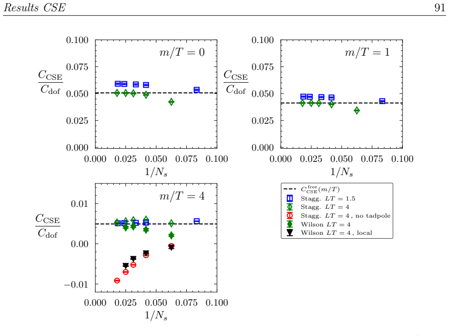
- [Fig. 4.2] The 'local' Wilson data points show a divergent continuum limit. Please add an explicit note in the caption or legend that this refers to the local vector current of Eq. (4.22), not to a local axial current, to avoid confusion.
- [Eqs. (4.10)-(4.13)] The relation between the 3-link current Γ_ν5 and the 5-link current Γ_ν Γ_5 is introduced only later. It would be clearer to define both operators at the same point and state explicitly that they are not identical at finite lattice spacing but share the same continuum limit.
- [Eq. (4.16)] The notation for the disconnected terms uses the same angle brackets for ensemble averages and for the factorized products. This is understandable but worth a remark in the text, especially because the tadpole term is the least familiar contribution.
- [Ch. 6] For the localized CME, a figure showing the spatial profile of the current alongside the volume-averaged value would be helpful. If such a figure already exists, please make the sign convention for the inhomogeneous field explicit in the caption.
Circularity Check
No significant circularity: results are measured and cross-checked against external benchmarks; self-citations and rooting are validation issues, not circular inputs.
full rationale
The thesis's derivation chain is self-contained in the relevant sense. The central CSE result (Ch. 4) is obtained by measuring the axial-current derivative eq. (4.16) on lattice ensembles and extracting CCSE from the slope versus eB (Fig. 4.1); it is then compared to the independent free-fermion formula (3.72) and to Wilson-fermion crosschecks in free and quenched systems (Secs. 4.2.2, 4.3.1, 4.3.2). No parameter is fitted to the target value and no observable is defined in terms of the claimed outcome. The CME result (Ch. 5) likewise follows from expectation values of the conserved vector current, with the non-zero local-current signal in the literature explicitly traced to the use of a non-conserved local current—an explanation, not a definitional equivalence. Bloch's theorem is an external input used as motivation, and the lattice measurement confirms rather than assumes it. The localized CME (Ch. 6) is a spatial profile measured in an inhomogeneous background; its zero volume average is consistent with, but not imposed by, the conserved-current Ward identity. The self-citations to Refs. [152] and [138] indicate the source papers of the presented data/methods and are not load-bearing for the physical argument. The main limitation—rooted staggered fermions for the full-QCD and localized-CME results (Sec. 2.6.2), with Wilson crosschecks only free/quenched—is an acknowledged correctness/validation gap, not a circular step: the rooting trick is an assumption about the lattice discretization, not a re-labelling of the target observable. Therefore no circularity is present.
Axiom & Free-Parameter Ledger
axioms (4)
- domain assumption Rooting trick for staggered fermions: the fourth root of the staggered fermion determinant describes one physical fermion flavor in the continuum limit.
- domain assumption Bloch's theorem generalizes to interacting QCD: a global conserved current vanishes in the equilibrium ground state.
- domain assumption The 3-link staggered axial current (Eq. 4.11) has the correct continuum limit for anomalous transport coefficients.
- standard math Standard lattice QCD framework: path integral, Wilson gauge action, Symanzik improvement, continuum limit via asymptotic freedom.
Cite this review
Pith. "Pith review of Lattice QCD Study of Anomalous Transport Phenomena in Strongly Interacting Matter." pith.science (2026). https://pith.science/paper/JS3NL3TJ
@misc{pith2026250906712,
  author       = {Pith},
  title        = {Pith review of: Lattice QCD Study of Anomalous Transport Phenomena in Strongly Interacting Matter},
  year         = {2026},
  howpublished = {\url{https://pith.science/paper/JS3NL3TJ}},
  note         = {Machine review of arXiv:2509.06712}
}
read the original abstract
In this thesis, we study the Chiral Magnetic Effect (CME) and the Chiral Separation Effect (CSE) using lattice QCD simulations. We completely characterize the CSE in QCD using $2+1$ simulations of staggered quarks tuned at the physical point. We find that the CSE conductivity is severely suppressed at low temperatures, and experiences a very sharp increase around the QCD crossover transition, reaching the value of massless non-interacting fermions at high temperatures. This is the first non-perturbative calculation of an anomalous transport conductivity in physical QCD. In the case of the CME, we show that this effect is not present in thermal equilibrium, in accordance with Bloch's theorem, both for free fermions and in QCD. We emphasize the crucial role of using a conserved vector current in the study of anomalous transport phenomena on the lattice, and how the use of non-conserved currents is behind non-vanishing results for the CME in equilibrium that can be found in the literature. Finally, we study the interplay between the CME and inhomogeneous magnetic fields, which leads us to find a novel localized CME signal in equilibrium. This does not contradict Bloch's theorem, since the total signal averages to zero when summed over the full volume. This effect is present in physical QCD, showing that a local equilibrium CME signal is possible in the presence of gluonic interactions.
Figures




Reference graph
Works this paper leans on
-
[1]
Question of parity conservation in weak interactions,
T. D. Lee and C. N. Yang, “Question of parity conservation in weak interactions,” Phys. Rev. 104 (Oct, 1956) 254–258. https://link.aps.org/doi/10.1103/PhysRev.104.254
-
[2]
Experimental test of parity conservation in beta decay,
C. S. Wu, E. Ambler, R. W. Hayward, D. D. Hoppes, and R. P. Hudson, “Experimental test of parity conservation in beta decay,”Phys. Rev. 105 (Feb,
-
[3]
Evidence for the2π decay of thek0 2 meson,
J. H. Christenson, J. W. Cronin, V. L. Fitch, and R. Turlay, “Evidence for the2π decay of thek0 2 meson,” Phys. Rev. Lett. 13 (Jul, 1964) 138–140. https://link.aps.org/doi/10.1103/PhysRevLett.13.138
-
[4]
Violation of CP Invariance, C asymmetry, and baryon asymmetry of the universe,
A. D. Sakharov, “Violation of CP Invariance, C asymmetry, and baryon asymmetry of the universe,”Pisma Zh. Eksp. Teor. Fiz. 5 (1967) 32–35
1967
-
[5]
R. F. Streater and A. S. Wightman,PCT, Spin and Statistics, and All That . Princeton University Press, 1989. http://www.jstor.org/stable/j.ctt1cx3vcq
1989
-
[6]
The Neutron EDM in the SM: A Review,
S. Dar, “The Neutron EDM in the SM: A Review,”arXiv:hep-ph/0008248
-
[7]
Improved experimental limit on the electric dipole moment of the neutron,
C. A. Baker, D. D. Doyle, P. Geltenbort, K. Green, M. G. D. van der Grinten, P. G. Harris, P. Iaydjiev, S. N. Ivanov, D. J. R. May, J. M. Pendlebury, J. D. Richardson, D. Shiers, and K. F. Smith, “Improved experimental limit on the electric dipole moment of the neutron,”Phys. Rev. Lett. 97 (Sep, 2006) 131801. https://link.aps.org/doi/10.1103/PhysRevLett.97.131801
-
[8]
TASI Lectures on the Strong CP Problem and Axions,
A. Hook, “TASI Lectures on the Strong CP Problem and Axions,”PoS TASI2018(2019) 004, arXiv:1812.02669 [hep-ph]
Pith/arXiv arXiv 2019
-
[9]
EQUILIBRIUM PARITY VIOLATING CURRENT IN A MAGNETIC FIELD,
A. Vilenkin, “EQUILIBRIUM PARITY VIOLATING CURRENT IN A MAGNETIC FIELD,” Phys. Rev. D 22 (1980) 3080–3084. 147 Bibliography 148
1980
-
[10]
K. Fukushima, D. E. Kharzeev, and H. J. Warringa, “The Chiral Magnetic Effect,” Phys. Rev. D 78 (2008) 074033, arXiv:0808.3382 [hep-ph]
Pith/arXiv arXiv 2008
-
[11]
’Strongly interacting matter in magnetic fields’: an overview,
D. E. Kharzeev, K. Landsteiner, A. Schmitt, and H.-U. Yee, “’Strongly interacting matter in magnetic fields’: an overview,”Lect. Notes Phys. 871 (2013) 1–11, arXiv:1211.6245 [hep-ph]
Pith/arXiv arXiv 2013
-
[12]
Quantum anomalies in dense matter,
D. T. Son and A. R. Zhitnitsky, “Quantum anomalies in dense matter,”Phys. Rev. D 70 (2004) 074018, arXiv:hep-ph/0405216
Pith/arXiv arXiv 2004
-
[13]
Anomalous axion interactions and topological currents in dense matter,
M. A. Metlitski and A. R. Zhitnitsky, “Anomalous axion interactions and topological currents in dense matter,”Phys. Rev. D 72 (2005) 045011, arXiv:hep-ph/0505072
Pith/arXiv arXiv 2005
-
[14]
D. E. Kharzeev and H.-U. Yee, “Chiral Magnetic Wave,”Phys. Rev. D 83 (2011) 085007, arXiv:1012.6026 [hep-th]
Pith/arXiv arXiv 2011
-
[15]
Fluid dynamics of R-charged black holes,
J. Erdmenger, M. Haack, M. Kaminski, and A. Yarom, “Fluid dynamics of R-charged black holes,”JHEP 01 (2009) 055, arXiv:0809.2488 [hep-th]
Pith/arXiv arXiv 2009
-
[16]
Hydrodynamics from charged black branes,
N. Banerjee, J. Bhattacharya, S. Bhattacharyya, S. Dutta, R. Loganayagam, and P. Surowka, “Hydrodynamics from charged black branes,”JHEP 01 (2011) 094, arXiv:0809.2596 [hep-th]
Pith/arXiv arXiv 2011
-
[17]
Holographic nonlinear hydrodynamics from AdS/CFT with multiple/non-Abelian symmetries,
M. Torabian and H.-U. Yee, “Holographic nonlinear hydrodynamics from AdS/CFT with multiple/non-Abelian symmetries,”JHEP 08 (2009) 020, arXiv:0903.4894 [hep-th]
Pith/arXiv arXiv 2009
-
[18]
Chiral Magnetic Effect in Heavy Ion Collisions: The Present and Future,
D. E. Kharzeev, J. Liao, and P. Tribedy, “Chiral Magnetic Effect in Heavy Ion Collisions: The Present and Future,”arXiv:2405.05427 [nucl-th]
-
[19]
Confinement of Quarks,
K. G. Wilson, “Confinement of Quarks,”Phys. Rev. D 10 (1974) 2445–2459
1974
-
[20]
Exact evolution equation for the effective potential,
C. Wetterich, “Exact evolution equation for the effective potential,”Phys. Lett. B 301 (1993) 90–94, arXiv:1710.05815 [hep-th]
Pith/arXiv arXiv 1993
-
[21]
QCD at finite temperature and chemical potential from Dyson–Schwinger equations,
C. S. Fischer, “QCD at finite temperature and chemical potential from Dyson–Schwinger equations,” Prog. Part. Nucl. Phys. 105 (2019) 1–60, arXiv:1810.12938 [hep-ph]
Pith/arXiv arXiv 2019
-
[22]
Holographic QCD: Past, Present, and Future,
Y. Kim, I. J. Shin, and T. Tsukioka, “Holographic QCD: Past, Present, and Future,” Prog. Part. Nucl. Phys. 68 (2013) 55–112, arXiv:1205.4852 [hep-ph] . Bibliography 149
Pith/arXiv arXiv 2013
-
[23]
Flavour Lattice A veraging Group (FLAG) Collaboration, Y. Aokiet al., “FLAG Review 2024,”arXiv:2411.04268 [hep-lat]
Pith/arXiv arXiv 2024
-
[24]
Muong − 2: Lattice calculations of the hadronic vacuum polarization,
S. Kuberski, “Muong − 2: Lattice calculations of the hadronic vacuum polarization,” PoS LATTICE2023(2024) 125, arXiv:2312.13753 [hep-lat]
Pith/arXiv arXiv 2024
-
[25]
Y. Aoki, G. Endrodi, Z. Fodor, S. D. Katz, and K. K. Szabo, “The Order of the quantum chromodynamics transition predicted by the standard model of particle physics,” Nature 443 (2006) 675–678, arXiv:hep-lat/0611014
Pith/arXiv arXiv 2006
-
[26]
The chiral and deconfinement aspects of the QCD transition,
A. Bazavovet al., “The chiral and deconfinement aspects of the QCD transition,” Phys. Rev. D 85 (2012) 054503, arXiv:1111.1710 [hep-lat]
Pith/arXiv arXiv 2012
-
[27]
The QCD equation of state with dynamical quarks,
S. Borsányi, G. Endrődi, Z. Fodor, A. Jakovác, S. D. Katz, S. Krieg, C. Ratti, and K. K. Szabó, “The QCD equation of state with dynamical quarks,”JHEP 11 (2010) 077, arXiv:1007.2580 [hep-lat]
Pith/arXiv arXiv 2010
-
[28]
Equation of state in ( 2+1 )-flavor QCD,
HotQCD Collaboration, A. Bazavovet al., “Equation of state in ( 2+1 )-flavor QCD,” Phys. Rev. D 90 (2014) 094503, arXiv:1407.6387 [hep-lat]
Pith/arXiv arXiv 2014
-
[29]
Montvay and G
I. Montvay and G. Munster,Quantum fields on a lattice . Cambridge Monographs on Mathematical Physics. Cambridge University Press, 3, 1997
1997
-
[30]
H. J. Rothe,Lattice Gauge Theories : An Introduction (Fourth Edition) , vol. 43. World Scientific Publishing Company, 2012
2012
-
[31]
Gattringer and C
C. Gattringer and C. B. Lang,Quantum chromodynamics on the lattice , vol. 788. Springer, Berlin, 2010
2010
-
[32]
M. E. Peskin and D. V. Schroeder,An Introduction to quantum field theory . Addison-Wesley, Reading, USA, 1995
1995
-
[33]
Laine and A
M. Laine and A. Vuorinen,Basics of Thermal Field Theory , vol. 925. Springer,
-
[34]
Susskind Fermions on a Euclidean Lattice,
H. S. Sharatchandra, H. J. Thun, and P. Weisz, “Susskind Fermions on a Euclidean Lattice,” Nucl. Phys. B 192 (1981) 205–236
1981
-
[35]
N. Sadooghi and H. J. Rothe, “Continuum behavior of lattice QED, discretized with one sided lattice differences, in one loop order,”Phys. Rev. D 55 (1997) 6749–6759, arXiv:hep-lat/9610001. Bibliography 150
Pith/arXiv arXiv 1997
-
[36]
Continuum Limit and Improved Action in Lattice Theories. 1. Principles andϕ4 Theory,
K. Symanzik, “Continuum Limit and Improved Action in Lattice Theories. 1. Principles andϕ4 Theory,” Nucl. Phys. B 226 (1983) 187–204
1983
-
[37]
Quantization of Nonabelian Gauge Theories,
V. N. Gribov, “Quantization of Nonabelian Gauge Theories,”Nucl. Phys. B 139 (1978) 1
1978
-
[38]
Meson masses in electromagnetic fields with Wilson fermions,
G. S. Bali, B. B. Brandt, G. Endrődi, and B. Gläßle, “Meson masses in electromagnetic fields with Wilson fermions,”Phys. Rev. D 97 no. 3, (2018) 034505, arXiv:1707.05600 [hep-lat]
Pith/arXiv arXiv 2018
-
[39]
M. D. Schwartz,Quantum Field Theory and the Standard Model . Cambridge University Press, 3, 2014
2014
-
[40]
Absence of Neutrinos on a Lattice. 1. Proof by Homotopy Theory,
H. B. Nielsen and M. Ninomiya, “Absence of Neutrinos on a Lattice. 1. Proof by Homotopy Theory,”Nucl. Phys. B 185 (1981) 20. [Erratum: Nucl.Phys.B 195, 541 (1982)]
1981
-
[41]
Absence of Neutrinos on a Lattice. 2. Intuitive Topological Proof,
H. B. Nielsen and M. Ninomiya, “Absence of Neutrinos on a Lattice. 2. Intuitive Topological Proof,” Nucl. Phys. B 193 (1981) 173–194
1981
-
[42]
S. D. Drell, M. Weinstein, and S. Yankielowicz, “Strong Coupling Field Theories
-
[43]
A Remnant of Chiral Symmetry on the Lattice,
P. H. Ginsparg and K. G. Wilson, “A Remnant of Chiral Symmetry on the Lattice,” Phys. Rev. D 25 (1982) 2649
1982
-
[44]
Exactly massless quarks on the lattice,
H. Neuberger, “Exactly massless quarks on the lattice,”Phys. Lett. B 417 (1998) 141–144, arXiv:hep-lat/9707022
Pith/arXiv arXiv 1998
-
[45]
Fermions and Gauge Fields on a Lattice,”Phys. Rev. D 14 (1976) 1627
1976
-
[46]
Lattice Fermions: Species Doubling, Chiral Invariance, and the Triangle Anomaly,
L. H. Karsten and J. Smit, “Lattice Fermions: Species Doubling, Chiral Invariance, and the Triangle Anomaly,”Nucl. Phys. B 183 (1981) 103
1981
-
[47]
Path Integral Measure for Gauge Invariant Fermion Theories,
K. Fujikawa, “Path Integral Measure for Gauge Invariant Fermion Theories,” Phys. Rev. Lett. 42 (1979) 1195–1198
1979
-
[48]
A Method for simulating chiral fermions on the lattice,
D. B. Kaplan, “A Method for simulating chiral fermions on the lattice,”Phys. Lett. B 288 (1992) 342–347, arXiv:hep-lat/9206013
Pith/arXiv arXiv 1992
-
[49]
New Phenomena in Subnuclear Physics: Proceedings, International School of Subnuclear Physics, Erice, Sicily, Jul 11-Aug 1 1975. Part A . Plenum, New York, USA, 1977. Bibliography 151
1975
-
[50]
Improved Continuum Limit Lattice Action for QCD with Wilson Fermions,
B. Sheikholeslami and R. Wohlert, “Improved Continuum Limit Lattice Action for QCD with Wilson Fermions,”Nucl. Phys. B 259 (1985) 572
1985
- [51]
-
[52]
Hamiltonian Formulation of Wilson’s Lattice Gauge Theories,
J. B. Kogut and L. Susskind, “Hamiltonian Formulation of Wilson’s Lattice Gauge Theories,” Phys. Rev. D 11 (1975) 395–408
1975
-
[53]
Effective Lagrangian and Dynamical Symmetry Breaking in Strongly Coupled Lattice QCD,
N. Kawamoto and J. Smit, “Effective Lagrangian and Dynamical Symmetry Breaking in Strongly Coupled Lattice QCD,”Nucl. Phys. B 192 (1981) 100
1981
-
[54]
Chiral Symmetry on the Lattice with Wilson Fermions,
M. Bochicchio, L. Maiani, G. Martinelli, G. C. Rossi, and M. Testa, “Chiral Symmetry on the Lattice with Wilson Fermions,”Nucl. Phys. B 262 (1985) 331
1985
-
[55]
Rooted staggered fermions: Good, bad or ugly?,
S. R. Sharpe, “Rooted staggered fermions: Good, bad or ugly?,”PoS LAT2006 (2006) 022, arXiv:hep-lat/0610094
Pith/arXiv arXiv 2006
-
[56]
Chiral anomalies and rooted staggered fermions,
M. Creutz, “Chiral anomalies and rooted staggered fermions,”Phys. Lett. B 649 (2007) 230–234, arXiv:hep-lat/0701018
Pith/arXiv arXiv 2007
-
[57]
New Phase Structure for Lattice QCD with Wilson Fermions,
S. Aoki, “New Phase Structure for Lattice QCD with Wilson Fermions,”Phys. Rev. D 30 (1984) 2653
1984
-
[58]
W. E. A. Verplanke, Z. Fodor, A. Gerardin, J. N. Guenther, L. Lellouch, K. K. Szabo, B. C. Toth, and L. Varnhorst, “Lattice QCD calculation of theη and η′ meson masses at the physical point using rooted staggered fermions,” arXiv:2409.18846 [hep-lat]
-
[59]
Perturbative improvement for lattice QCD: An Update,
P. Lepage, “Perturbative improvement for lattice QCD: An Update,”Nucl. Phys. B Proc. Suppl. 60 (1998) 267–278, arXiv:hep-lat/9707026
Pith/arXiv arXiv 1998
-
[60]
Physics ofη′ with rooted staggered quarks,
S. Durr, “Physics ofη′ with rooted staggered quarks,”Phys. Rev. D 85 (2012) 114503, arXiv:1203.2560 [hep-lat]
Pith/arXiv arXiv 2012
-
[61]
The Equation of state in lattice QCD: With physical quark masses towards the continuum limit,
Y. Aoki, Z. Fodor, S. D. Katz, and K. K. Szabo, “The Equation of state in lattice QCD: With physical quark masses towards the continuum limit,”JHEP 01 (2006) 089, arXiv:hep-lat/0510084
Pith/arXiv arXiv 2006
-
[62]
Chemical Potential on the Lattice,
P. Hasenfratz and F. Karsch, “Chemical Potential on the Lattice,”Phys. Lett. B 125 (1983) 308–310. Bibliography 152
1983
-
[63]
Analytic smearing of SU(3) link variables in lattice QCD,
C. Morningstar and M. J. Peardon, “Analytic smearing of SU(3) link variables in lattice QCD,” Phys. Rev. D 69 (2004) 054501, arXiv:hep-lat/0311018
Pith/arXiv arXiv 2004
-
[64]
Thermodynamics of SU(3) lattice gauge theory,
G. Boyd, J. Engels, F. Karsch, E. Laermann, C. Legeland, M. Lutgemeier, and B. Petersson, “Thermodynamics of SU(3) lattice gauge theory,”Nucl. Phys. B 469 (1996) 419–444, arXiv:hep-lat/9602007
Pith/arXiv arXiv 1996
-
[65]
G. Aarts et al., “Phase Transitions in Particle Physics: Results and Perspectives from Lattice Quantum Chromo-Dynamics,”Prog. Part. Nucl. Phys. 133 (2023) 104070, arXiv:2301.04382 [hep-lat]
Pith/arXiv arXiv 2023
-
[66]
Wuppertal-Budapest Collaboration, S. Borsanyi, Z. Fodor, C. Hoelbling, S. D. Katz, S. Krieg, C. Ratti, and K. K. Szabo, “Is there still anyTc mystery in lattice QCD? Results with physical masses in the continuum limit III,”JHEP 09 (2010) 073, arXiv:1005.3508 [hep-lat]
Pith/arXiv arXiv 2010
-
[67]
The QCD phase diagram for external magnetic fields,
G. S. Bali, F. Bruckmann, G. Endrődi, Z. Fodor, S. D. Katz, S. Krieg, A. Schäfer, and K. K. Szabó, “The QCD phase diagram for external magnetic fields,”JHEP 02 (2012) 044, arXiv:1111.4956 [hep-lat]
Pith/arXiv arXiv 2012
-
[68]
QCD with background electromagnetic fields on the lattice: a review,
G. Endrodi, “QCD with background electromagnetic fields on the lattice: a review,” arXiv:2406.19780 [hep-lat]
-
[69]
QCD phase diagram with isospin chemical potential,
B. B. Brandt and G. Endrődi, “QCD phase diagram with isospin chemical potential,” PoS LATTICE2016(2016) 039, arXiv:1611.06758 [hep-lat]
Pith/arXiv arXiv 2016
-
[70]
QCD phase diagram and equation of state in background electric fields,
G. Endrodi and G. Marko, “QCD phase diagram and equation of state in background electric fields,”Phys. Rev. D 109 no. 3, (2024) 034506, arXiv:2309.07058 [hep-lat]
Pith/arXiv arXiv 2024
-
[71]
Scaling Laws and Triviality Bounds in the Lattice phi**4 Theory. 1. One Component Model in the Symmetric Phase,
M. Luscher and P. Weisz, “Scaling Laws and Triviality Bounds in the Lattice phi**4 Theory. 1. One Component Model in the Symmetric Phase,”Nucl. Phys. B 290 (1987) 25–60
1987
-
[72]
On electric fields in hot QCD: perturbation theory,
G. Endrődi and G. Markó, “On electric fields in hot QCD: perturbation theory,” JHEP 12 (2022) 015, arXiv:2208.14306 [hep-ph]
Pith/arXiv arXiv 2022
-
[73]
Scaling Laws and Triviality Bounds in the Lattice phi**4 Theory. 3. N Component Model,
M. Luscher and P. Weisz, “Scaling Laws and Triviality Bounds in the Lattice phi**4 Theory. 3. N Component Model,”Nucl. Phys. B 318 (1989) 705–741. Bibliography 153
1989
-
[74]
Is there a Landau pole problem in QED?,
M. Gockeler, R. Horsley, V. Linke, P. E. L. Rakow, G. Schierholz, and H. Stuben, “Is there a Landau pole problem in QED?,”Phys. Rev. Lett. 80 (1998) 4119–4122, arXiv:hep-th/9712244
Pith/arXiv arXiv 1998
-
[75]
Scaling Laws and Triviality Bounds in the Lattice phi**4 Theory. 2. One Component Model in the Phase with Spontaneous Symmetry Breaking,
M. Luscher and P. Weisz, “Scaling Laws and Triviality Bounds in the Lattice phi**4 Theory. 2. One Component Model in the Phase with Spontaneous Symmetry Breaking,” Nucl. Phys. B 295 (1988) 65–92
1988
-
[76]
Review of particle physics,
Particle Data Group Collaboration, S. Navaset al., “Review of particle physics,” Phys. Rev. D 110 no. 3, (2024) 030001
2024
-
[77]
Current algebra and some nonstrong mesonic decays,
D. G. Sutherland, “Current algebra and some nonstrong mesonic decays,”Nucl. Phys. B 2 (1967) 433–440
1967
-
[78]
R. Sommer, “Scale setting in lattice QCD,”PoS LATTICE2013(2014) 015, arXiv:1401.3270 [hep-lat]
Pith/arXiv arXiv 2014
-
[79]
Axial vector vertex in spinor electrodynamics,
S. L. Adler, “Axial vector vertex in spinor electrodynamics,”Phys. Rev. 177 (1969) 2426–2438
1969
-
[80]
A PCAC puzzle:π0 →γγ in theσ model,
J. S. Bell and R. Jackiw, “A PCAC puzzle:π0 →γγ in theσ model,” Nuovo Cim. A 60 (1969) 47–61
1969
discussion (0)
Sign in with ORCID, Apple, or X to comment. Anyone can read and Pith papers without signing in.