REVIEW 3 major objections 5 minor 19 references
Visualizing RNN States with Predictive Semantic Encodings
T0 review · 3 major / 5 minor · reviewed 2026-08-14 · deepseek-v4-flash
Pith's one-line read An RNN state's meaning reduces to its next-word odds
desk verdict A modest, clearly written PSE visualization idea whose load-bearing 'state semantics as probability distribution' claim is only validated for the output state; the memory-state conclusions need a probe-family control. read the letter →
The pith
A machine-rendered reading of the paper's core claim, the machinery that carries it, and where it could break.
The reading
What carries the argument
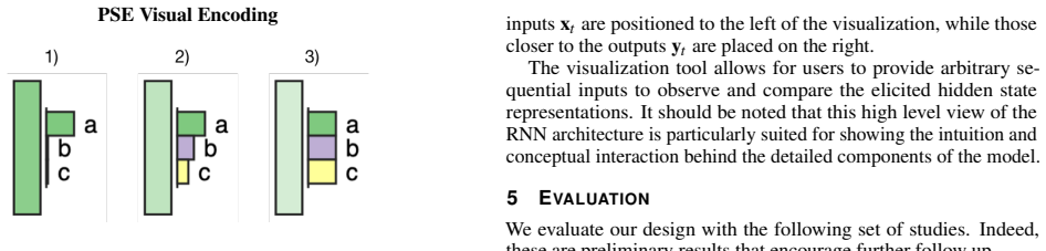
The central object is the Predictive Semantic Encoding (PSE), defined as the context-free function $G(\gamma, v)$ that produces a probability distribution over the task's outputs $y$ for a given hidden state kind $\gamma$ and instance $v$; the RNN's own classifier $F(h)$ is the specialization where $\gamma$ is the final hidden state. $G$ is trained separately, with its own parameters for every hidden state kind, after the original RNN finishes training. The PSE does two kinds of work: it maps all hidden states into a common output space so they can be compared visually and quantitatively, and its predictive accuracy as measured by perplexity doubles as a measure of how much of a state's meaning survives without surrounding context.
What would settle it
Find a held-out sentence and a timestep where the LSTM's own output distribution assigns high probability to the actual next word but the Output-state PSE assigns it near-zero probability; if such discordant cases occur systematically across the test set, the claim that PSEs are accurate generalizations of the classifier $F$ would be refuted.
Extended reading notes
Core claim
The central claim is that a hidden state's semantics can be represented by its predicted effect: PSEs express the meaning of hidden states in relation to task inputs or outputs, via a context-free function $G(\gamma, v)$ that maps a hidden state $v$ of kind $\gamma$ to a probability distribution over output labels $y$. The RNN's own output classifier $F(h)$ is a special case, $G(\gamma, h)$ with $\gamma$ the final hidden state, so the encoding and the task share a visual and mathematical space. The authors demonstrate on a two-layer LSTM language model that the 2nd-layer Output state PSE reaches test perplexity 70 against the RNN's 66.5, establishing parity with $F$, while Long-term Memory and Cell states score orders of magnitude worse. They explain the gap as those states carrying information that must be combined with other context before it becomes a prediction, and they use the encoded distributions to trace how uncertainty at the end of a quotation resolves into a confident verb prediction after the word she.
Load-bearing premise
The load-bearing assumption is that a fixed, context-free function trained on one hidden state kind in isolation, $G(\gamma, v)$, fairly represents that state's meaning; the paper's own results show this fails for Long-term Memory and Cell states, which the authors attribute to those states depending on other context.
Editorial extensions
If this is right
- All hidden state kinds can be placed side by side at any timestep, since each is encoded as the same kind of next-output distribution; the authors use this to show which LSTM components are pointing toward a verb versus a noun.
- Because PSE perplexity tracks how self-contained a state's semantics are, the encoding gives a quantitative signal for where information in the LSTM is context-dependent; the paper identifies Long-term Memory and Cell states as exactly such states.
- The PSE can be trained after the fact on an already trained RNN, so the technique offers a way to inspect existing language models without retraining or architectural changes.
- Since the PSE shares the output representation with the task, visualizations can combine hidden state encodings with model outputs and part-of-speech colourings, foregrounding shifts in grammatical prediction across timesteps.
Reading between the lines
- An implication the authors leave implicit is that PSE perplexity could serve as a general diagnostic for gating design: comparing these scores across architectures would quantify which components carry context-dependent information.
- The paper mentions predicting outputs at varying timesteps but does not evaluate it; one testable extension is training PSEs to predict words two or three steps ahead and checking whether distributions sharpen at consistent points in a sentence.
- The visual case study reads a change in PSE colours as the Short-term Memory switching the model to a verb prediction, but PSEs are correlational summaries; treating those readings as hypotheses and testing them with gate ablations is a natural follow-up the paper does not perform.
Signed reviews
Editorial analysis
A structured set of objections, weighed in public.
Referee Report
Summary. The paper introduces Predictive Semantic Encodings (PSE), a technique that represents each hidden state of an LSTM as a probability distribution over the language model's output vocabulary. A separate context-free classifier G(γ, v) is trained per hidden state kind to map that state's vector to a next-word distribution, and the resulting distributions are displayed with a color rectangle and a mini-bar chart in a proof-of-concept visualization tool. The authors evaluate PSE accuracy on the Penn Treebank language modeling task with a 2-layer LSTM, reporting that the Output state's PSE reaches a test perplexity of 70 versus the RNN's 66.5, while Long-term Memory and Cell states have much higher perplexities, which they interpret as reflecting genuine semantic ambiguity. A case study of the sentence "we stand in solidarity," she emphasized. is used to illustrate how the visualization reveals information flow across LSTM gates.
Significance. The idea of summarizing hidden states as output distributions is simple and potentially useful: it provides a common, task-aligned representation that allows visual comparison across different LSTM components. The paper gives a concrete quantitative evaluation on a standard benchmark and is transparent that the results are preliminary. If the central interpretation is valid, the technique could be a lightweight addition to RNN analysis toolkits. However, the evidence as presented does not yet secure the claim that PSEs express the meaning of hidden states 'as a whole': the quantitative validation rests on a single probe class, and the visualization's utility is supported only by a narrative case study, not by a user study or task-based evaluation.
major comments (3)
- [§4.2, §5.2, Figure 3] The inference that Long-term Memory and Cell states are 'highly ambiguous' because their PSE perplexities are orders of magnitude worse than the Output state conflates linear probe failure with absence of semantics. The authors define G(γ,v) as a context-free function and evaluate it only with a simple linear classifier. A high-perplexity result could mean either that the state genuinely lacks standalone predictive content or that the state's content is not linearly decodable without context. No control distinguishes these hypotheses; e.g., an MLP probe or a probe that conditions on the neighboring hidden states (such as the cell input or output gate) would disambiguate them. Because Section 5.1 interprets the white, flat PSEs for c2_6, c2_7, and l2_7 in Figure 1 as meaningful ambiguity, the unvalidated identification of linear decodability with semantic content is load-bearing for the paper's central claim.
- [§5.2] The claim that the Output state PSE perplexity of 70 is 'on par' with the RNN's 66.5 is supported only by a single point estimate. No error bars, confidence intervals, or significance tests are reported, so the size of the gap (3.5 perplexity points) is not interpretable. The authors should provide repeated training runs or bootstrap intervals, and ideally compare against a trivial baseline (e.g., a frequency-based unigram model) to show that the linear probe is capturing signal beyond chance. Without this, the parity claim, which underpins the statement that PSEs are an 'accurate generalization' of the RNN classifier, is unsubstantiated.
- [§5.1] The case study is a post-hoc narrative with no validation against alternative explanations or baseline visualizations. For example, the claim that l2_8 'is still retaining semantics which indicate a noun prediction' and that the Output Gate switches the semantic to a verb is presented as fact, but there is no quantitative measure of how reliable these PSE differences are, nor any comparison to a random or shuffled PSE baseline. Since the paper's contribution is a visualization technique, the absence of any user study or task-based evaluation leaves the core utility claim untested. At minimum, the authors should frame Section 5.1 as an illustrative example and explicitly outline a validation plan (e.g., a controlled experiment with Architects/Trainers) as future work.
minor comments (5)
- [Equation (1)] The perplexity formula is written as 'T √' which is ambiguous; it should be the T-th root of the product. Also, the text below the equation says 'P(xt|xt ...xt−1)', which is a typo for 'P(xt|x1...xt−1)' or 'P(xt|w1...wt−1)' as in the formula itself.
- [Abstract and §1] The phrase 'deep nature' to describe RNNs is imprecise; LSTM cells have depth in the unrolled sense, but calling them 'deep' in the first sentence may mislead readers.
- [§2, Reference [1]] The author name 'Y . V . Bengio' appears to have a typo; it should be 'Y. Bengio'.
- [§4.2] The description 'top-k as 10% of the vocabulary' is unclear because k should be an integer; the authors should specify how the 10% threshold is rounded or state that they show the top 10% of classes.
- [§5.1] The text contains 'who's' where 'whose' is meant (the language model, who's outputs).
Circularity Check
PSE semantics are defined as the output of a fitted linear probe, so the conclusion that high-perplexity states are semantically ambiguous partly restates that definition.
-
self definitional
[Section 4.2 (semantic definition) applied in Section 5.2 (interpretation of Figure 3)]
"We recall from the previous section the desire to express the intuitions encoded within RNN hidden states as a whole. To do so, we introduce the semantics of hidden states as a probability distribution over the task output labels. More formally, we consider the context free function G(γ, v) which produces a probability distribution over the outputs y, where γ denotes the specific kind of hidden state of the instance v."
Section 4.2 defines hidden-state semantics as the probability distribution output by the trained context-free function G. Consequently, the PSE visualization is, by construction, a plot of a fitted classifier's output; there is no independent quantity called 'semantics' being measured. Section 5.2 then reports that Long-term Memory and Cell states have very high PSE perplexity and concludes that their semantics are 'highly ambiguous' and that these states 'naturally bear little stand-alone representational power.' But the only evidence is the poor perplexity of the very function used to define the semantics. If semantics were defined differently, high linear PSE perplexity would not by itself show ambiguity.
full rationale
The paper is not built on a self-citation chain: the only self-reference is to its own supplemental material [15], and that citation is not load-bearing. The central 'derivation' is a design choice: PSE is defined by the authors as the probability distribution produced by a separately trained function G (Section 4.2). The held-out perplexity measurement for the second-layer Output state (70 versus 66.5) is a real sanity check that G can approximate the RNN's classifier; that part is not circular. The circularity is partial and localized to interpretation: because 'semantics' was defined as G's output, the paper's conclusion that Long-term Memory and Cell states are semantically ambiguous (Section 5.2) is partly a restatement of G's high perplexity for those states. The empirical contrast among state kinds is genuine, but the paper does not test whether a different probe class or added context would recover those states' content, so the 'ambiguity' conclusion is not independent of the chosen operationalization. That is a definitional circularity in the interpretive claim, not in the reported numbers, so the score is moderate rather than extreme.
Assumptions & free parameters
free parameters (2)
- PSE linear classifier weights per hidden state kind =
not reported (weight matrices per state kind)
- top-k fraction for visual encoding =
10% of vocabulary
assumptions (3)
- domain assumption A hidden state's semantics can be represented as a context-free probability distribution over task outputs via a separately trained function G.
- ad hoc to paper A linear classifier is sufficient for G to capture the semantics relevant for comparison.
- domain assumption Perplexity on held-out next-word prediction is an appropriate measure of semantic fidelity for a visualization.
invented entities (1)
-
Predictive Semantic Encoding (PSE)
Cite this review
Pith. "Pith review of Visualizing RNN States with Predictive Semantic Encodings." pith.science (2026). https://pith.science/paper/JSDF2F7O
@misc{pith2026190800588,
  author       = {Pith},
  title        = {Pith review of: Visualizing RNN States with Predictive Semantic Encodings},
  year         = {2026},
  howpublished = {\url{https://pith.science/paper/JSDF2F7O}},
  note         = {Machine review of arXiv:1908.00588}
}
read the original abstract
Recurrent Neural Networks are an effective and prevalent tool used to model sequential data such as natural language text. However, their deep nature and massive number of parameters pose a challenge for those intending to study precisely how they work. We present a visual technique that gives a high level intuition behind the semantics of the hidden states within Recurrent Neural Networks. This semantic encoding allows for hidden states to be compared throughout the model independent of their internal details. The proposed technique is displayed in a proof of concept visualization tool which is demonstrated to visualize the natural language processing task of language modelling.
Figures


Reference graph
Works this paper leans on
-
[1]
D. Bahdanau, K. Cho, and Y . Bengio. Neural machine translation by jointly learning to align and translate. arXiv preprint arXiv:1409.0473, 2014
arXiv 2014
-
[2]
T. Bolukbasi, K.-W. Chang, J. Y . Zou, V . Saligrama, and A. T. Kalai. Man is to computer programmer as woman is to homemaker? debiasing word embeddings. In Advances in neural information processing systems, pp. 4349–4357, 2016
work page 2016
-
[3]
D. Cashman, G. Patterson, A. Mosca, and R. Chang. Rnnbow: Vi- sualizing learning via backpropagation gradients in recurrent neural networks. In Workshop on Visual Analytics for Deep Learning (VADL), vol. 4, 2017
work page 2017
-
[4]
Hochreiter and J
S. Hochreiter and J. Schmidhuber. Long short-term memory. Neural computation, 9(8):1735–1780, 1997
1997
- [5]
-
[6]
A. Karpathy, J. Johnson, and L. Fei-Fei. Visualizing and understanding recurrent networks. arXiv preprint arXiv:1506.02078, 2015
arXiv 2015
-
[7]
O. Levy, K. Lee, N. FitzGerald, and L. Zettlemoyer. Long short-term memory as a dynamically computed element-wise weighted sum.arXiv preprint arXiv:1805.03716, 2018
work page Pith review arXiv 2018
-
[8]
J. Li, X. Chen, E. Hovy, and D. Jurafsky. Visualizing and understanding neural models in nlp. arXiv preprint arXiv:1506.01066, 2015
arXiv 2015
Show all 19 references
-
[9]
J. Li, W. Monroe, and D. Jurafsky. Understanding neural networks through representation erasure. arXiv preprint arXiv:1612.08220 , 2016
2016 arXiv
-
[10]
Marcus, B
M. Marcus, B. Santorini, and M. A. Marcinkiewicz. Building a large annotated corpus of english: The penn treebank. 1993
1993
-
[11]
Mikolov, M
T. Mikolov, M. Karafi´at, L. Burget, J. ˇCernock`y, and S. Khudanpur. Recurrent neural network based language model. In Eleventh annual conference of the international speech communication association , 2010
2010
-
[12]
Y . Ming, S. Cao, R. Zhang, Z. Li, Y . Chen, Y . Song, and H. Qu. Understanding hidden memories of recurrent neural networks. In 2017 IEEE Conference on Visual Analytics Science and Technology (VAST) , pp. 13–24. IEEE, 2017
2017
-
[13]
T. Munzner. A nested model for visualization design and validation. IEEE transactions on visualization and computer graphics , 15(6):921– 928, 2009
2009
-
[14]
M. T. Ribeiro, S. Singh, and C. Guestrin. Why should i trust you?: Explaining the predictions of any classifier. In Proceedings of the 22nd ACM SIGKDD international conference on knowledge discovery and data mining, pp. 1135–1144. ACM, 2016
2016
-
[15]
Sawatzky
L. Sawatzky. Visualizing rnn states with predictive semantic encodings - supplemental material, Jul 2019
2019
-
[16]
Strobelt, S
H. Strobelt, S. Gehrmann, M. Behrisch, A. Perer, H. Pfister, and A. M. Rush. Seq-2-seq-vis: A visual debugging tool for sequence-to-sequence models. IEEE transactions on visualization and computer graphics , 25(1):353–363, 2019
2019
-
[17]
Strobelt, S
H. Strobelt, S. Gehrmann, H. Pfister, and A. M. Rush. Lstmvis: A tool for visual analysis of hidden state dynamics in recurrent neural networks. IEEE transactions on visualization and computer graphics , 24(1):667–676, 2018
2018
-
[18]
Sutskever, O
I. Sutskever, O. Vinyals, and Q. V . Le. Sequence to sequence learning with neural networks. In Advances in neural information processing systems, pp. 3104–3112, 2014
2014
-
[19]
D. Tang, B. Qin, and T. Liu. Document modeling with gated recurrent neural network for sentiment classification. In Proceedings of the 2015 conference on empirical methods in natural language processing , pp. 1422–1432, 2015. APPENDIX : L ONG SHORT-T ERM MEMORY The recurrence f...
2015
Reviewed August 14, 2026 · model on record in the stance chip above.
Discussion (0). Continue with ORCID to comment.