To Each Metric Its Decoding: Post-Hoc Optimal Decision Rules of Probabilistic Hierarchical Classifiers

Alexandre Perez-Lebel; Antoine Saillenfest; Matthieu Labeau; Roman Plaud; Thomas Bonald

REVIEW 3 major objections 4 minor 22 references

To Each Metric Its Decoding: Post-Hoc Optimal Decision Rules of Probabilistic Hierarchical Classifiers

T0 review · 3 major / 4 minor · reviewed 2026-08-07 · deepseek-v4-flash

Challenge this review Re-run · record.json Download PDF Read on arXiv ↗

Pith's one-line read The paper proves that any hierarchical classifier can be decoded exactly for a wide class of metrics in near-linear time, and that hierarchical F-scores can be optimized over exponentially large prediction sets.

desk verdict A genuinely useful decoding framework with a correct core, but Theorem 4.7's proof has gaps and the complexity claim needs correction before it is fully trustworthy. read the letter →

arxiv 2506.01552 v1 pith:JUEE6EBR submitted 2025-06-02 cs.LG stat.ML

Roman Plaud , Alexandre Perez-Lebel , Matthieu Labeau , Antoine Saillenfest , Thomas Bonald This is my paper

classification cs.LGstat.ML

keywords hierarchicalclassificationBayes-optimaldecodingcost-sensitivedecisionruleF-scoretreedistancelossnodeprobabilitypost-hocinferenceunderdeterminedprediction

verification ladder T0 review T1 audit T2 compute T3 formal

The pith

A machine-rendered reading of the paper's core claim, the machinery that carries it, and where it could break.

The reading

The paper aims to settle how to read out a prediction from a probabilistic hierarchical classifier: instead of heuristics like top-leaf argmax, it derives the Bayes-optimal decision rule for the metric you actually care about. It proves that for any 'hierarchically reasonable' metric over nodes, the expected-cost-minimizing node can be found in $O(d_{\max} |L| + |N|)$ time, and for hierarchical $F_\beta$ scores over sets of nodes in $O(d_{\max}^2 |N|)$ time. This matters because decoding is usually decoupled from evaluation; the same posterior distribution should be decoded differently depending on whether you optimize tree distance, Wu-Palmer similarity, or hF1. Experiments on image hierarchies show that optimal decoding consistently outperforms common heuristics, and the gap widens when inputs are blurred and the posterior becomes underdetermined.

What carries the argument

The load-bearing object is the node probability $p(n)=\sum_{l\in L(n)} p(l)$, the bottom-up mass of a node's leaf descendants, together with the node-parent loss difference $\delta^C_{nl}=C(n,l)-C(\pi(n),l)$. For hierarchically reasonable metrics, the sign of $\delta^C_{nl}$ is fixed by whether the true label lies under $n$, which yields per-node thresholds $q^{C}_{\min}(n)$ and $q^{C}_{\max}(n)$. Lemma 4.3 prunes $n$ or its parent when $p(n)$ falls outside these thresholds, and a level-counting argument bounds the survivor set by $O(d_{\max})$. For $hF_\beta$, the closed form $hF_\beta(h,l)=(1+\beta^2)|h\cap A(l)|/(|h|+\beta^2(d(l)+1))$ makes the expected utility additive over nodes, so the optimizer reduces to a top-$k$ selection over weights $\Delta^\beta_k(n)$.

What would settle it

Take a small complete binary tree, generate a random posterior $p$ and a random hierarchically reasonable cost matrix (or use $hF_\beta$ for any $\beta$), compute the optimal decision by exhaustive enumeration of all nodes or all maximal antichains, and compare it with the paper's algorithms; a single mismatch would refute Theorem 4.4 or 4.7. A cheaper targeted test for Lemma 4.3 is to search over cost matrices satisfying (2)-(3) for a node $n$ with $p(n)$ outside $[q_{\min}(n), q_{\max}(n)]$ whose expected cost is still minimal.

Watch

Extended reading notes

Core claim

Given a tree hierarchy over classes and a posterior distribution over its leaves, the Bayes-optimal prediction relative to a cost metric $C$ is the minimizer of expected cost. The paper shows that this minimizer can be found without enumerating all nodes: for metrics satisfying a monotonicity condition called hierarchical reasonableness, node $n$ is provably suboptimal unless its subtree probability $p(n)$ lies between two thresholds, and pruning on those thresholds leaves only $O(d_{\max})$ surviving candidates, giving Theorem 4.4. For the hierarchical F-score family, restricting predictions to maximal antichains and decomposing by $|h_{\text{aug}}|$ reduces the exponential search to selecting the top-$k$ nodes by additive weights $\Delta^\beta_k(n)$, giving Theorem 4.7. Empirically, the optimal rules beat eight heuristic decodings across six hierarchical metrics, with the largest gains on deliberately blurred images.

Load-bearing premise

The load-bearing premise is that the metric is 'hierarchically reasonable'—predicting a child is strictly worse than predicting its parent when the truth is outside the child's subtree and strictly better when inside—and that the posterior probabilities are exact; if the metric violates that ordering, the pruning that gives the speed guarantee can discard the true optimum.

Editorial extensions

If this is right

For any cost matrix satisfying the two monotonicity inequalities (2)-(3), the optimal node prediction becomes computable in $O(d_{\max}|L|+|N|)$ time instead of the $O(|N||L|)$ brute-force search.
The hierarchical $F_\beta$ score over node subsets, whose search space is exponential, is maximized exactly in $O(d_{\max}^2|N|)$ time, making set-valued 'hesitation' predictions tractable.
Decoding is metric-specific: the same posterior can legitimately lead to different optimal predictions (leaf, internal node, or set of nodes), and leaf argmax is Bayes-optimal only for the Top1 error.
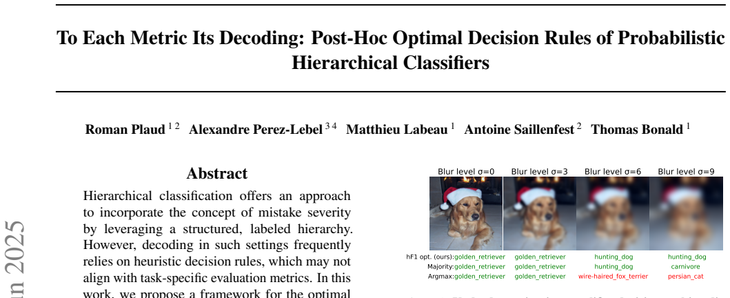
On image hierarchies, the optimal decoding strategies consistently beat eight heuristic strategies across six metrics, and the relative gains grow as the posterior becomes more uncertain, for example under image blurring.
The proposed algorithms run in a few microseconds to milliseconds per sample and are about 60 times faster than brute-force node decoding, while solving set-decoding problems that brute force cannot handle at all.

Reading between the lines

Editorial extensions of the paper, not claims the author makes directly.

Because the node algorithm works for any metric satisfying the ordering inequalities, the same pruning machinery could be reused for user-supplied cost matrices in applications like medical triage, once the metric is certified hierarchically reasonable.
The $hF_\beta$ set-decoding recipe resembles Bayes-optimal top-$k$ selection for flat F-measures; a natural extension is to derive similar additive weights for other set metrics such as hierarchical Jaccard or Hamming loss.
The optimality statements assume an oracle posterior; with a miscalibrated model, the decoded prediction is optimal only relative to estimated probabilities, so combining these decoders with hierarchical recalibration is a direct next step that the paper names.
Non-tree hierarchies (DAGs) are flagged as future work; the level-counting argument that bounds the candidate set by depth would need a different invariant for DAGs.

Share X Bluesky LinkedIn Reddit HN

Editorial analysis

A structured set of objections, weighed in public.

Desk editor's note, referee report, and a circularity audit.

Desk Editor's Note

read the letter

To my eye, this paper earns its place. The core contribution is a general, efficient optimal-decoding framework for hierarchical metrics, plus the first exact polynomial-time optimizer for hierarchical F_beta set predictions. Theorem 4.4 is clean: it recovers the known majority and generalized-threshold rules as special cases, and the pruning argument is solid. The experiments are broad and honest, and the blurring experiment actually demonstrates the claimed effect: when the posterior is near the center of the simplex, heuristic decodings lose ground to the optimal rule.

The soft spots are in the proof and presentation of Theorem 4.7, not in the core idea. The top-k reduction is justified by a monotonicity that is true but never stated: Delta^k(n) is a sum of nonnegative contributions over leaf descendants, so an ancestor always has at least as large a value. Without stating that, the reduction looks like a leap. Lemma E.13 has a genuine gap: it removes an arbitrary node n from the optimal set and applies the hF_beta formula that only holds for ancestor-closed sets. The argument only works if n is maximal in the set, and the paper doesn't say that. That is fixable. The complexity claim is the most serious issue. The algorithm as written enumerates k from 1 to |Q(p)| and does a top-k selection for each k, which costs O(|Q(p)|^2) = O(d_max^4). The stated O(d_max^2 |N|) is only valid when d_max^2 <= |N|; for typical balanced hierarchies this holds, but the theorem should say so or the algorithm should be changed. The text also says 'a few microseconds per sample' while Appendix D.3 reports about a millisecond for hF_beta; that inconsistency should be corrected.

None of these undercut the value of the contribution. The right call is to send to a serious referee, expect revision, and be willing to accept after the proof is tightened. I'd cite this paper if I work in hierarchical classification, and I'd bring it to reading group.

Referee Report

3 major / 4 minor

Summary. The paper develops a Bayes-optimal decoding framework for hierarchical classifiers: given a posterior distribution over leaf classes and a target evaluation metric, it seeks the prediction minimizing (or maximizing) expected metric value. It treats three prediction spaces: leaves, arbitrary nodes, and sets of nodes. For node predictions it introduces 'hierarchically reasonable' metrics and proves a pruning-based algorithm with claimed complexity O(d_max |L| + |N|), recovering known optimal rules for tree distance and generalized tree distance losses. For set predictions it focuses on hierarchical F-beta scores and claims a polynomial algorithm with complexity O(d_max^2 |N|), based on a reduction to top-k node selection. The empirical section compares the proposed decodings with several heuristics on TieredImageNet-H and iNat19 across many models, and includes controlled blurring experiments to test the claim that underdetermination increases the gap between optimal and heuristic decoding.

Significance. If the theoretical claims are correct, the paper provides a useful unifying view: several existing optimal decoding rules become special cases of one framework, and the hF-beta decoding problem is shown to be solvable in polynomial time despite an exponential candidate space. The empirical study is broad and unusually honest: the gains over heuristics are reported as modest (1-5% for most metrics), and the blurring experiments directly test the proposed explanation for when optimal decoding matters. The paper also makes a concrete reproducibility effort by releasing code. The main reservations concern the proof and complexity statement of the hF-beta theorem; these are load-bearing, but they appear fixable without changing the paper's scope.

major comments (3)

[Section 4.3 / Theorem 4.7, and Appendix E.2.4, Eq. (10) and Algorithm 12] The reduction to top-k selection is not justified as written. In Eq. (10) the maximization is over h_k in U_T(N) with h_k subset of Q(p), i.e., over ancestor-closed sets, but the proposed algorithm simply takes the k nodes in Q(p) with largest Delta^k(n). This is valid only if the resulting top-k set is itself ancestor-closed, which requires a monotonicity statement such as Delta^k(pi(n)) >= Delta^k(n) for every node n. The paper neither states nor proves this property. Without it, the algorithm can output a set that is not in the feasible domain, and the utility formula used in the proof does not apply to such a set. This is the step that turns an exponential search into a polynomial one, so it is central to the paper's main set-decoding claim.
[Appendix E.2.4, Lemma E.13] The proof of Lemma E.13 removes an arbitrary node n from an optimal set xi* and compares U(xi*) with U(xi* \ {n}). If n has descendants in xi*, then xi* \ {n} is not in U_T(N), and the formula for the utility (which assumes an ancestor-closed set) does not apply. The argument is only valid when n is a maximal node of xi*. To establish the lemma's conclusion xi* subset Q(p), one needs an additional argument showing that if any node in xi* violates p(n) < q_min(n), then a maximal node in xi* also violates it; this is likely true because the violation propagates to descendants (p decreases and q increases along downward paths), but it is not present in the manuscript. This is a gap in the proof of optimality of the hF-beta algorithm.
[Theorem 4.7 and proof of Theorem E.15] The complexity statement is not supported by the described algorithm. The proof explicitly states that the final step enumerates k in {1,...,|Q(p)|} and for each k finds the top-k elements among |Q(p)| in O(|Q(p)|) operations, giving O(d_max^4) for that step alone, and then concludes an overall complexity of O(d_max^2 |N|). This conclusion is valid only under an additional unstated assumption such as |N| >= d_max^2, which holds for bushy hierarchies but not for all trees satisfying the paper's setup (for example, a caterpillar-like tree has |N| = O(d_max)). The theorem should be restated with the more precise bound O(d_max^4 + d_max^2 |N|), or the algorithm should be refined to avoid the per-k top-k cost, or the extra assumption should be stated explicitly.

minor comments (4)

[Section 5.2 vs. Appendix D.3] The main text says decoding takes 'a few microseconds per sample', while Table D.7 reports times on the order of a millisecond for the hF-beta decodings (e.g., about 1.05 ms for hF1 on iNat19) and about 13 ms for the Zhao similarity decoding; this inconsistency should be corrected.
[Appendix E.2.4, Lemma E.12] The definition 'dmin = max_{l in L} d(l)' contradicts the intended meaning of dmin as the minimum leaf depth; the symbol should be min_{l in L} d(l) throughout Section E.2.4.
[Appendix E.2.3, Proposition E.11] The proposition uses argmin for an expected utility that is being maximized; this should be argmax.
[Abstract and code link] The GitHub URL in the abstract is broken by a line break ('hierarchical decision rules' contains a space in the rendered text); the URL should be a single link.

Circularity Check

0 steps flagged · score 0.0 of 10

No significant circularity: the optimal-rule derivations follow directly from expected-risk minimization, with known results recovered as corollaries and no fitted parameters.

full rationale

The paper's core derivations are self-contained. Definition 3.4 defines the optimal decision rule as the pointwise minimizer of the conditional expected cost E[C(h,y)|x], and each algorithm is obtained by algebraic manipulation of that same objective. Lemma 4.3 derives pruning thresholds q_min and q_max from the user-supplied cost matrix C; these are not fitted to data and do not presuppose the optimum. Lemma 4.6 derives q_hFbeta_min from beta and tree depths only. The known closed-form rules for tree-distance loss and generalized tree-distance loss are recovered as corollaries in Appendix E.1.2, which is independent supporting evidence rather than circularity. The hFbeta cardinality decomposition follows the external approach of Waegeman et al. (2014), and the utility rewriting in Equation (8) is an algebraic identity. The single self-citation (Plaud et al., 2024) appears in related work as a pointer to an alternative evaluation methodology and is not load-bearing for any theorem. Appendix B and the conclusion honestly restrict the optimality claims to oracle posteriors, which is a limitation, not a circular step. The reviewer-flagged gap in Theorem 4.7's proof—the top-k reduction needs an unstated monotonicity or maximal-node argument to ensure the selected set is ancestor-closed—is a correctness or completeness concern, not a circular reduction, so it does not raise the circularity score.

Assumptions & free parameters 0 free parameters · 3 assumptions · 0 invented entities

The central algorithms introduce no fitted constants: thresholds qC_min and qC_max are deterministic functions of the metric and tree, and q_hFbeta_min is a closed form of beta and depth. The proofs rely on standard probability and tree properties. The main domain assumption is the 'hierarchically reasonable' condition on the cost metric; it is stated explicitly but limits universality. Another assumption is tree-structured hierarchy. The oracle-posterior assumption is used in the theory and relaxed in experiments via plug-in estimates. No new entities (particles, forces, dimensions) are postulated.

assumptions (3)

domain assumption The evaluation metric C is hierarchically reasonable: for each node n, C(n,l) > C(pi(n),l) when l is outside L(n), and C(n,l) < C(pi(n),l) when l is inside L(n) (or the relaxed (3)-(4) form).
Invoked in Definition 4.2 and used in Lemma 4.3 to derive the q_min and q_max thresholds that enable O(d_max) pruning. If a metric violates these inequalities, the candidate set may exclude the optimal node, so Theorem 4.4 does not apply.
domain assumption The label hierarchy is a rooted tree T=(N,E) with leaves equal to the class set L.
All algorithms traverse parent-child relations and compute ancestor closures; Section 4 and the notation table assume a tree. Non-tree hierarchies are listed as future work.
domain assumption The posterior distribution over leaves is known exactly (oracle) for the optimality proofs.
Section 3.1 states that the authors assume the true posterior probability distribution. The empirical section relaxes this by plugging in model estimates, for which optimality is conditional on calibration.

how reviews work

0 comments

Cite this review

Pith. "Pith review of To Each Metric Its Decoding: Post-Hoc Optimal Decision Rules of Probabilistic Hierarchical Classifiers." pith.science (2026). https://pith.science/paper/JUEE6EBR

@misc{pith2026250601552,
  author       = {Pith},
  title        = {Pith review of: To Each Metric Its Decoding: Post-Hoc Optimal Decision Rules of Probabilistic Hierarchical Classifiers},
  year         = {2026},
  howpublished = {\url{https://pith.science/paper/JUEE6EBR}},
  note         = {Machine review of arXiv:2506.01552}
}

abstract

Hierarchical classification offers an approach to incorporate the concept of mistake severity by leveraging a structured, labeled hierarchy. However, decoding in such settings frequently relies on heuristic decision rules, which may not align with task-specific evaluation metrics. In this work, we propose a framework for the optimal decoding of an output probability distribution with respect to a target metric. We derive optimal decision rules for increasingly complex prediction settings, providing universal algorithms when candidates are limited to the set of nodes. In the most general case of predicting a subset of nodes, we focus on rules dedicated to the hierarchical $hF_{\beta}$ scores, tailored to hierarchical settings. To demonstrate the practical utility of our approach, we conduct extensive empirical evaluations, showcasing the superiority of our proposed optimal strategies, particularly in underdetermined scenarios. These results highlight the potential of our methods to enhance the performance and reliability of hierarchical classifiers in real-world applications. The code is available at https://github.com/RomanPlaud/hierarchical_decision_rules

Figures

Figures reproduced from arXiv: 2506.01552 by the authors.

**Figure 1.** Underdetermination amplifies decision-making disparities between decoding strategies. Predictions of three decoding strategies based on the probability estimates of a pretrained VGG11 model, for images with blur levels σ ∈ {0, 3, 6, 9}. Correct predictions are highlighted in green, incorrect in red. broader superclasses (Deng et al., 2009; Chang et al., 2021). The severity of a misclassification error is then rel… view at source ↗

**Figure 2.** Relative Gain (in %) of Decoding Strategies. Each dot represents the relative gain of the optimal strategy vs. the average over all other strategies for a specific metric and model on the test set of a given dataset, with symbols indicating the dataset: ▲ for models pretrained on ImageNet, ⋆ for models fine-tuned on ImageNet-H, and • for models fine-tuned on iNat19. Boxplots summarize the distribution of relative ga… view at source ↗

**Figure 3.** Agreement map on the simplex of R 3 for two decoding strategies. For a hierarchy with three leaf nodes displayed in the top-left corner, this figure shows the agreement map between hF1 and Majority decoding : each point p in the simplex is color-coded, a green dot indicates equality of the two predictions, while a red dot indicates a disagreement. I(n) = log( |L| |L(n)| ) to define these strategies. These can be cat… view at source ↗

Discussion (0). Sign in to comment.

Reference graph

Works this paper leans on

22 extracted references · 19 canonical work pages

[1]

p(n) > M n M n+mn := qC max(n) = ⇒ ξ∗ C(p) ̸= π(n)

work page
[2]

Let L : N × L →R satisfy Equations (2) and (3)

p(n) < mn mn+Mn := qC min(n) = ⇒ ξ∗ C(p) ̸= n Proof. Let L : N × L →R satisfy Equations (2) and (3). We now proceed to prove statement 1. Assume p(n) > M n M n+mn . Then, we have: p(n) > M n M n + mn ⇐ ⇒ mn p(n)|{z} =P l∈L(n) p(l) > Mn (1 − p(n))| {z } =P l∈L\L(n) p(l) This implies X l∈L(n) p(l) · mn|{z} ≤C(π(n),l)−C(n,l) > X l∈L\L(n) p(l) · M n|{z} ≥C(n,...

work page
[3]

This is independant of the input probability distribution p and can be performed beforehand

A brute-force algorithm is performed on this remaining candidate set (Algorithm 5) • Algorithm 2 correspond to the computation of (qC min(n))n∈N and (qC max(n))n∈N . This is independant of the input probability distribution p and can be performed beforehand. To this extent, the time complexity of Algorithm 1 is not added to the overall complexity of the o...

work page 2015
[4]

For each k in {1

∆ computation. For each k in {1 . . .|Q(p)|}, ∆(k) is computed through a tree traversal in which each node is visited exactly once. Therefore this step has a O(|Q(p)| · |N |) = O(d2 max · |N |)

work page
[5]

|Q(p)|}

The last step consists in enumerating all k ∈ {1 . . .|Q(p)|}. Each step requires first to find the top k elements of among |Q(p)| which can be performed in |Q(p)| operation and then compute the sum this k element. Overall each step has then a O(|Q(p)| + k) = O(|Q(p)|) = O(d2 max) time complexity. Then, in total the total complexity is O(d4 max) In total ...

work page
[7]

(Algorithm 3)

Computing probability distribution over nodes, given probability distribution over leaves. (Algorithm 3)

work page
[8]

It outputs a candidate set S which can all be the optimal prediction (Algorithm 4)

Filtering each node based on condition of Lemma E.2. It outputs a candidate set S which can all be the optimal prediction (Algorithm 4)

work page
[10]

p(n) > ˜M n ˜M n+ ˜mn · p(an) :=qC max(n) · p(an) =⇒ ξ∗ C (p) ̸= π(n)

work page

Show all 22 references

[11]

Let L : N × L →R be a hierarchical metric that satisfy Equations (3) and (4)

p(n) < ˜mn ˜mn+ ˜Mn · p(an) :=qC min(n) · p(an) =⇒ ξ∗ C (p) ̸= n Proof. Let L : N × L →R be a hierarchical metric that satisfy Equations (3) and (4). We now proceed to prove statement 2. Assume p(n) < ˜mn ˜mn+ ˜Mn p(an). Then, we have: p(n) < ˜mn ˜mn + ˜Mn p(an) ⇐ ⇒ ˜Mn p(n)|{...
[12]

(Algorithm 3)

Compute probability distribution over nodes, given probability distribution over leaves. (Algorithm 3)
[13]

It outputs a candidate set S which can all be the optimal prediction (Algorithm 7)

Filtering each node based on condition of Theorem E.6. It outputs a candidate set S which can all be the optimal prediction (Algorithm 7)
[14]

Let us now prove that |S| = O(dmax)

A brute-force algorithm is performed on this remaining candidate set (Algorithm 5) As before, We obtain a O(|S| · |L|+ |N |) time complexity for Algorithm 8. Let us now prove that |S| = O(dmax). We recall second condition 2 of Proposition E.6: p(n) < qC min(n) · p(an) = ⇒ ξ∗ C...

2014
[15]

We obtain Q(p) and compute ∆β k (n) for k ≤ |Q(p)| and n ∈ Q(p)
[16]

For each k ≤ |Q(p)|, we find h∗ k which consists in the k nodes that correspond to the top- k (∆β k (n))n∈Q(p) and compute UhFβ (h∗ k|p) = P n∈h∗ k ∆β k (n)
[17]

We find optimal rule with kopt = maxk≤|Q(p)| UhFβ (h∗ k|p) and ξ∗ hFβ (p) = h∗ kopt 42 To Each Metric Its Decoding: Post-Hoc Optimal Decision Rules of Probabilistic Hierarchical Classifiers Algorithm 9 Computation of depths 1: function DREC(n, δ, d) 2: if n ∈ Lthen 3: d(n) ← δ...
[18]

This is performed through a tree traversal which visit exactly once each node

Node probability computation. This is performed through a tree traversal which visit exactly once each node. Therefore the time complexity is O(|N |)
[19]

Similarly, it is a tree traversal which has O(|N |) time complexity

Depths computation. Similarly, it is a tree traversal which has O(|N |) time complexity
[20]

This is also performed through a tree traversal which visit at most each node one

Q(p) computation. This is also performed through a tree traversal which visit at most each node one. Therefore the time complexity is O(|N |). This three first steps can be performed simultaneously. For convenience, we separate to make it more understandable
[1973]

Amigo, E

URL https://www.fq.math.ca/Scanned/ 11-4/aho-a .pdf. Amigo, E. and Delgado, A. Evaluating extreme hierarchical multi-label classification. In Muresan, S., Nakov, P., and Villavicencio, A. (eds.), Proceedings of the 60th Annual Meeting of the Association for Computational Lingu...

2022
[1999]

Dosovitskiy, A., Beyer, L., Kolesnikov, A., Weissenborn, D., Zhai, X., Unterthiner, T., Dehghani, M., Minderer, M., Heigold, G., Gelly, S., Uszkoreit, J., and Houlsby, N

doi: 10 .1145/312129.312220. Dosovitskiy, A., Beyer, L., Kolesnikov, A., Weissenborn, D., Zhai, X., Unterthiner, T., Dehghani, M., Minderer, M., Heigold, G., Gelly, S., Uszkoreit, J., and Houlsby, N. An image is worth 16x16 words: Transformers for image recognition at scale. I...

2021
[2001]

ISBN 158113391X

Association for Computing Machinery. ISBN 158113391X. doi: 10 .1145/502512.502540. URL https://doi.org/10.1145/502512.502540. Zhao, H., Torralba, A., Torresani, L., and Yan, Z. Open vocabulary scene parsing. In Proceedings of the IEEE International Conference on Computer Visio...

2018
[2017]

Ren, M., Triantafillou, E., Ravi, S., Snell, J., Swersky, K., Tenenbaum, J

doi: 10 .1109/CVPR.2017.690. Ren, M., Triantafillou, E., Ravi, S., Snell, J., Swersky, K., Tenenbaum, J. B., Larochelle, H., and Zemel, R. S. Meta-learning for semi-supervised few-shot classifica- tion. In International Conference on Learning Repre- sentations, 2018. URL https...

2017 arXiv

Pith tools

Reviewed August 7, 2026 · model on record in the stance chip above.

[1] [1]

p(n) > M n M n+mn := qC max(n) = ⇒ ξ∗ C(p) ̸= π(n)

work page

[2] [2]

Let L : N × L →R satisfy Equations (2) and (3)

p(n) < mn mn+Mn := qC min(n) = ⇒ ξ∗ C(p) ̸= n Proof. Let L : N × L →R satisfy Equations (2) and (3). We now proceed to prove statement 1. Assume p(n) > M n M n+mn . Then, we have: p(n) > M n M n + mn ⇐ ⇒ mn p(n)|{z} =P l∈L(n) p(l) > Mn (1 − p(n))| {z } =P l∈L\L(n) p(l) This implies X l∈L(n) p(l) · mn|{z} ≤C(π(n),l)−C(n,l) > X l∈L\L(n) p(l) · M n|{z} ≥C(n,...

work page

[3] [3]

This is independant of the input probability distribution p and can be performed beforehand

A brute-force algorithm is performed on this remaining candidate set (Algorithm 5) • Algorithm 2 correspond to the computation of (qC min(n))n∈N and (qC max(n))n∈N . This is independant of the input probability distribution p and can be performed beforehand. To this extent, the time complexity of Algorithm 1 is not added to the overall complexity of the o...

work page 2015

[4] [4]

For each k in {1

∆ computation. For each k in {1 . . .|Q(p)|}, ∆(k) is computed through a tree traversal in which each node is visited exactly once. Therefore this step has a O(|Q(p)| · |N |) = O(d2 max · |N |)

work page

[5] [5]

|Q(p)|}

The last step consists in enumerating all k ∈ {1 . . .|Q(p)|}. Each step requires first to find the top k elements of among |Q(p)| which can be performed in |Q(p)| operation and then compute the sum this k element. Overall each step has then a O(|Q(p)| + k) = O(|Q(p)|) = O(d2 max) time complexity. Then, in total the total complexity is O(d4 max) In total ...

work page

[6] [7]

(Algorithm 3)

Computing probability distribution over nodes, given probability distribution over leaves. (Algorithm 3)

work page

[7] [8]

It outputs a candidate set S which can all be the optimal prediction (Algorithm 4)

Filtering each node based on condition of Lemma E.2. It outputs a candidate set S which can all be the optimal prediction (Algorithm 4)

work page

[8] [10]

p(n) > ˜M n ˜M n+ ˜mn · p(an) :=qC max(n) · p(an) =⇒ ξ∗ C (p) ̸= π(n)

work page