A Finite-Difference Trust-Region Method for Convexly Constrained Smooth Optimization

D\^an\^a Davar; Geovani Nunes Grapiglia

REVIEW 2 major objections 5 minor 31 references

A Finite-Difference Trust-Region Method for Convexly Constrained Smooth Optimization

T0 review · 2 major / 5 minor · reviewed 2026-08-04 · deepseek-v4-flash

Challenge this review Re-run · record.json Download PDF Read on arXiv ↗ Review JSON

Pith's one-line read A derivative-free trust-region method matches known complexity bounds for convexly constrained smooth optimization.

desk verdict A solid, clean DFO trust-region result with honest proofs; the real soft spot is a gap between the theorem's sufficient-decrease condition and the FISTA-based implementation, plus an unenforced bounded-Hessian assumption. read the letter →

arxiv 2510.17366 v2 pith:K2LOSZNA submitted 2025-10-20 math.OC

Dânâ Davar , Geovani Nunes Grapiglia This is my paper · ORCID

classification math.OC MSC 90C3090C56

keywords derivative-freeoptimizationtrust-regionmethodsfinite-differenceapproximationsworst-casecomplexityconvexconstraintsPolyak-Lojasiewiczfunctionsfunctionevaluationbound

verification ladder T0 review T1 audit T2 compute T3 formal

The pith

A machine-rendered reading of the paper's core claim, the machinery that carries it, and where it could break.

The reading

The paper proposes TRFD-S, a derivative-free trust-region method that approximates gradients by forward finite differences, builds quadratic models with an approximate Hessian, and solves only one trust-region subproblem per iteration. Its central claim is that this single-subproblem design attains the best known finite-difference evaluation-complexity rates while handling convex constraints and without ever computing a separate stationarity measure. Specifically, it proves O(n (L/(σε))^{-2}) evaluations for nonconvex objectives to reach an (L/σ)ε-approximate stationary point, O(n (L/(σε))^{-1}) evaluations for convex objectives to reduce the functional residual below Δmax(L/σ)ε, and O(n log((L/(σε))^{-1})) evaluations for Polyak–Lojasiewicz functions on R^n. The bounds depend on a user-supplied estimate σ of the Lipschitz constant L, which creates an explicit accuracy–cost tradeoff. This matters because it shows that the simpler, cheaper-per-iteration design need not sacrifice the theoretical efficiency of finite-difference trust-region methods, extending those guarantees to convexly constrained black-box problems.

What carries the argument

The central mechanism is the coupling between the finite-difference stepsize τ_k and the trust-region radius Δ_k: the update rules maintain τ_k√n ≤ Δ_k at every iteration, which forces the gradient approximation error to satisfy ∥∇f(x_k) − g_k∥ ≤ (L/2)Δ_k. This bound lets the method control the gap between the true stationarity measure ψ_{Δmax} and the approximate η_{Δmax}, and turns the standard trust-region acceptance test into a sufficient-decrease argument that uses η_{Δmax} only in proofs, not in computations. The user-supplied Lipschitz estimate σ sets the target tolerance (L/σ)ε and the initial stepsize τ0 = ε/(σ√n), producing the explicit tradeoff captured in the complexity bounds.

What would settle it

Run TRFD-S on a low-dimensional convex problem with a deliberately weak subproblem solver that stops at any feasible point without enforcing the Cauchy decrease; if the number of evaluations to reach the predicted functional residual exceeds the proven O(n(L/(σε))^{-1}) bound—or the trust-region radius keeps halving to machine precision—then condition (4) is not satisfied by that solver.

Watch

Extended reading notes

Core claim

The paper claims that TRFD-S—a trust-region method using finite-difference gradient approximations, quadratic models, and one subproblem solve per iteration—needs at most O(n (L/(σε))^{-2}) function evaluations to reach an (L/σ)ε-approximate stationary point on a closed convex set, O(n (L/(σε))^{-1}) evaluations when f is convex to drive the functional residual below Δmax(L/σ)ε, and O(n (L/µ) log((σ/L)(f(x0)−f*)/εf)) evaluations for Polyak–Lojasiewicz functions on R^n. These bounds hold even though the method never computes the approximate stationarity measure η; the only requirement is that each subproblem step delivers a Cauchy-type sufficient decrease (condition (4)). The paper also gives

Load-bearing premise

The complexity theorems assume every subproblem step satisfies a sufficient-decrease condition (4) involving a stationarity measure the algorithm never computes, and that the Hessian approximations stay uniformly bounded; if a practical solver violates (4) or H_k grows without bound, the proven evaluation counts do not apply.

Editorial extensions

If this is right

For smooth nonconvex problems with convex constraints, derivative-free trust-region methods can match the O(n ε^{-2}) evaluation complexity of unconstrained finite-difference methods, up to a factor (σ/L)^2.
For convex objectives, the O(n ε^{-1}) rate provides a linear-in-budget accuracy guarantee without needing a separate stationarity measure computation.
The Polyak–Lojasiewicz logarithmic bound extends derivative-free fast rates to non-strongly-convex functions on unconstrained domains.
The unrelaxable-bound variant inherits the same worst-case guarantees, so box-constrained black-box problems enjoy the proven bounds.
The parameter σ acts as a dial: overestimating L gives stricter accuracy at higher worst-case cost, while underestimating L lowers cost but weakens the achievable accuracy guarantee.

Reading between the lines

Editorial extensions of the paper, not claims the author makes directly.

The explicit σ-tradeoff suggests an online adaptation strategy—start with a modest overestimate of L and decrease it as the run progresses—which the paper does not explore but which could reduce average evaluation cost while preserving final accuracy.
The unrelaxable-bound construction uses one-sided differences near the boundary; a natural extension would be to general closed convex sets via projected finite-difference steps, though the paper only treats boxes.
The constants in the bounds depend on a uniform bound M on ∥H_k∥ that the safeguarded BFGS update does not explicitly enforce; proving boundedness of that update would close the gap between the theory and the tested implementation.
The single-subproblem design indicates that the earlier two-subproblem TRFD scheme can be simplified for smooth problems without losing the logarithmic rate for Polyak–Lojasiewicz functions.

Share X Bluesky LinkedIn Reddit HN

Editorial analysis

A structured set of objections, weighed in public.

Desk editor's note, referee report, and a circularity audit.

Desk Editor's Note

read the letter

Worth a look if you work on derivative-free methods or evaluation complexity. The new piece is TRFD-S, which combines quadratic models, finite-difference gradients, Cauchy-type decrease, and convex constraints in one trust-region subproblem per iteration, avoiding the second subproblem that TRFD needs for a stationarity measure. The complexity results are the expected targets: O(n ε^{-2}) for nonconvex, O(n ε^{-1}) for convex, O(n log ε^{-1}) for P-L functions on unconstrained domains, all matching the best finite-difference rates for unconstrained smooth problems while handling convex feasible sets. I checked the main proof chain—Lemmas 3.3 through 3.8, the convex and P-L analogues—and the inequalities are coherent. Constants track, the tolerance scaling with L/σ is explicit, and no fitted values are hidden in the bounds. That is a genuine and useful contribution to the DFO complexity literature.

The soft spots are real but not fatal to the theory. First, condition (4) in Step 2 requires the trial step to give a Cauchy-type decrease measured with η_{Δmax}(x_k), which is never computed. The paper cites the generalized Cauchy step as sufficient, and for unconstrained problems TRSgep plausibly returns something good enough. But the bound-constrained experiments use FISTA with Dykstra projections, and no proof is offered that FISTA's finite output satisfies (4). So those numerical results are not formally covered by Corollaries 3.10 and 3.17. This is an implementation-coverage gap, not a contradiction in the theorems. Second, Assumption A3 (uniformly bounded H_k) is assumed without an algorithmic safeguard; the "safeguarded" BFGS rule merely skips updates when ⟨s_k,y_k⟩≤0, which does not keep the norm bounded. The M-dependent constants in Δ_min and β are therefore not guaranteed for the code. Both issues are fixable, but they should be fixed before publication.

Who gets value: anyone doing worst-case complexity analysis for derivative-free methods, and people using trust-region DFO solvers with constraints. The math is solid enough that I'd send it to peer review, but I'd ask the authors to close the gap between Algorithm 1's hypotheses and the tested implementation—either by proving the actual subproblem solver satisfies (4), or by modifying the algorithm to compute an explicit generalized Cauchy step, and by adding a genuine safeguard on H_k. My inclination is conditional acceptance with those revisions.

Referee Report

2 major / 5 minor

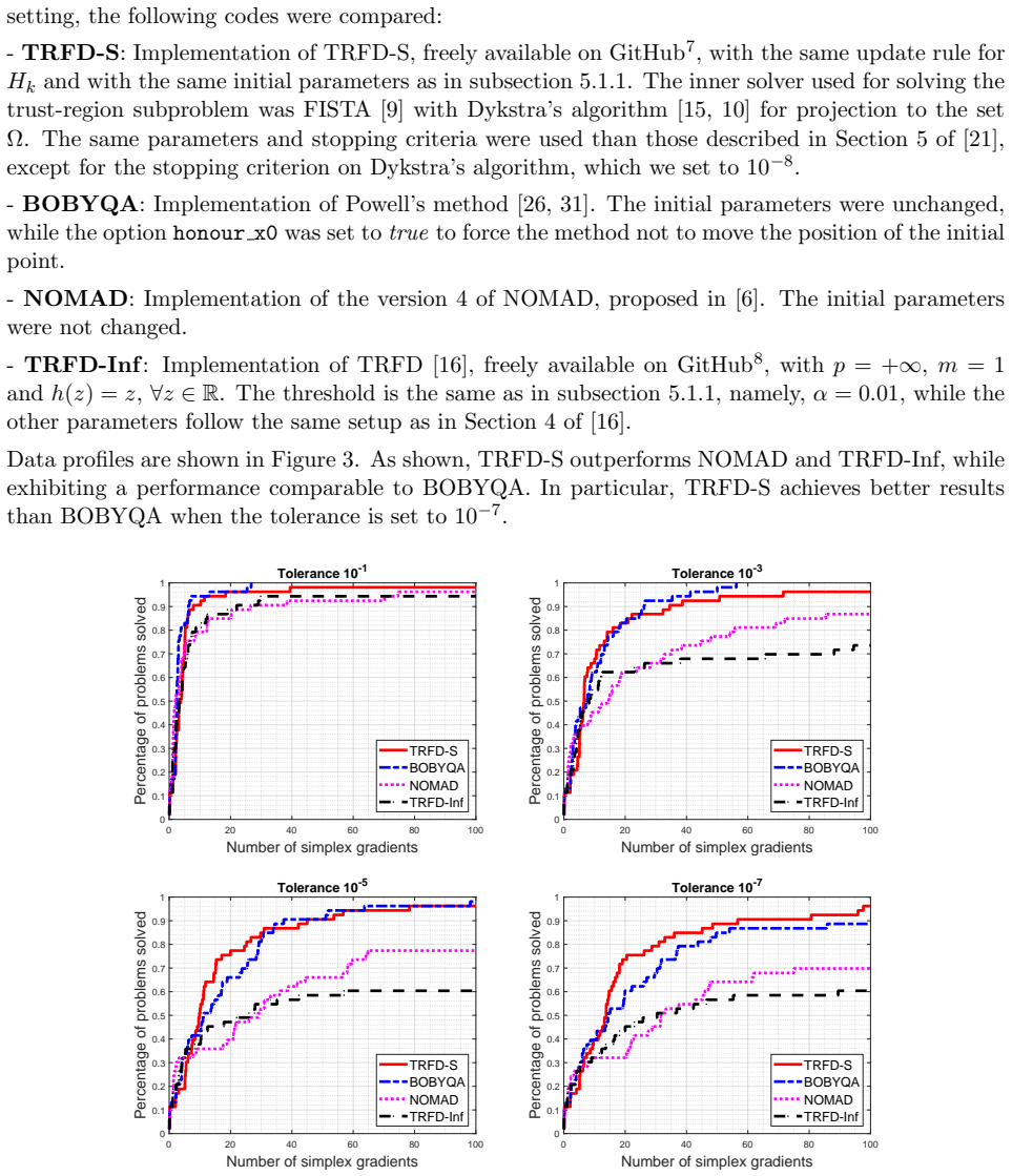
Summary. The paper proposes TRFD-S, a derivative-free trust-region method that uses forward finite-difference gradient approximations and quadratic models for smooth optimization over closed convex sets. It proves worst-case evaluation-complexity bounds: for nonconvex objectives, O(n (L/(σ ε))^{-2}) evaluations to reach an (L/σ)ε-approximate stationary point; for convex objectives, O(n (L/(σ ε))^{-1}) evaluations to reach a Δmax(L/σ)ε-approximate minimizer; and for Polyak–Lojasiewicz objectives on R^n, O(n log(((L/(σ ε))^{-1}))) evaluations. The method avoids a separate stationarity-measure subproblem. An adaptation for unrelaxable box constraints is given, and numerical experiments compare TRFD-S with NEWUOA, DFQRM, TRFD, BOBYQA, and NOMAD.

Significance. If the theorems are correct, the paper extends finite-difference trust-region complexity guarantees from unconstrained to convexly constrained smooth problems without computing a stationarity measure, matching the best known finite-difference rates in the unconstrained case. The proof chain is explicit and the constants are tracked, and the manuscript ships a MATLAB implementation with benchmark data-profiling code, which strengthens reproducibility. The main contributions are valuable, but the theoretical guarantees are conditional on two assumptions that the implemented algorithm does not demonstrably enforce: the sufficient-decrease condition (4) for the subproblem solver and the Hessian bound A3 for the safeguarded BFGS update.

major comments (2)

[Algorithm 1, Step 2; Remark 3.1; §5.1.2] Condition (4) is load-bearing for every complexity result (Lemmas 3.7, 3.14, 3.20 and Theorems 3.9, 3.16, 3.22). The algorithm requires the subproblem solver to return a step satisfying (4), but the paper never computes η_Δmax(x_k) and gives no proof that the implemented solvers do so. For the unconstrained experiments TRSgep returns an exact trust-region solution, so (4) plausibly holds with κ=1/2. For the bound-constrained experiments in §5.1.2, the subproblem is solved by FISTA with Dykstra projections, an approximate first-order method, and no argument is given that its finite output satisfies (4). Since the generalized Cauchy step guarantee in Remark 3.1 is only asserted, the numerical results on the More–Wild bound-constrained set are not formally covered by Corollaries 3.10 and 3.17. Please provide a proof of (4) for the constrained subproblem solver, or modify the algorithm to co
[Assumption A3; §5.1.1] The complexity bounds use the constant M through Δmin in Lemma 3.6, β in Lemma 3.13, and γ in Lemma 3.19. The safeguarded BFGS update in §5.1.1 is not shown to keep ∥H_k∥ ≤ M. The condition |⟨s_k,y_k⟩|>0 only avoids division by zero; it does not ensure positive curvature or boundedness of the Hessian approximation. If H_k becomes unbounded, all M-dependent constants in the proofs cease to be valid for the implementation. Please add an explicit safeguarding step (e.g., a projection or scaling of H_k to enforce ∥H_k∥≤M) in the algorithm, or prove that the stated BFGS update maintains boundedness under the algorithm's dynamics.

minor comments (5)

[Algorithm 1, Step 4] The line 'Define x_{k+1}=x_k and Δ_{k+1}=...' is missing the 'Step 4' label; this is a typographical issue.
[Table 3] The table heading says 'strongly convex problems', but A7 is the Polyak–Lojasiewicz condition, which is more general than strong convexity. Change the heading to 'P-L functions' for accuracy.
[§5.1.1] The definition of the user parameter σ appears garbled: 'σ= ϵ√n√eps'. Please clarify whether it is ε√n/√eps or ε√n√eps, and state the corresponding units/scaling.
[Lemma 3.3, proof] After bounding 1−ρ_k, the proof says 'by (8) we get Δ_k < η_Δmax(x_k)/∥H_k∥'. Since the minimum in the denominator is then attained by Δ_k, it would be clearer to display this step explicitly, as the reader must otherwise reconstruct the min.
[Corollary 3.10] The asymptotic expression in (26) drops the M term that appears in the explicit bound (25). Please state that the O notation treats M as a constant, or include M in the displayed rate.

Circularity Check

0 steps flagged · score 0.0 of 10

No significant circularity: the complexity theorems are conditional derivations from explicit assumptions; sigma is a user-set parameter, not a fitted constant, and no prediction is equivalent to an input by construction.

full rationale

I walked the derivation chain for Theorems 3.9, 3.16, 3.22 and Corollaries 3.10, 3.17, 3.23. Each iteration bound is obtained from the sufficient-decrease hypothesis (4), the finite-difference error bound (7), the stationarity-measure comparison (Lemma 3.5), and the trust-region update rules. None of these steps reduces to the conclusion. The factor (L/sigma)epsilon appears on both sides of the statements because tau0 = epsilon/(sigma*sqrt(n)) is chosen so that the finite-difference gradient error is O(L epsilon/sigma); hence (L/sigma)epsilon is the natural accuracy scale. sigma is a user input, not a quantity fitted to any data or to the target value. The lemmas cited from the authors' earlier TRFD paper [16] are prior published auxiliary results used inside otherwise new proofs; there is no uniqueness theorem or ansatz smuggled in via self-citation that forces the present conclusions. The numerical experiments against NEWUOA, BOBYQA, NOMAD, DFQRM and TRFD provide external benchmark support. Two manuscript-noted gaps are correctness/coverage risks, not circularity: Remark 3.1 states that 'TRFD-S never computes eta_{Delta_max}(x_k)' and condition (4) is guaranteed only if the subproblem solver returns at least a generalized Cauchy step, while the FISTA-based solver used for bound constraints is not shown to do so; and Assumption A3 (||H_k|| <= M) is assumed, but the safeguarded BFGS update in Section 5.1.1 is not shown to preserve that bound. These make the results conditional but do not make the claims true by construction.

Assumptions & free parameters 4 free parameters · 8 assumptions · 0 invented entities

The bounds are proven, not fitted: the only user-chosen quantity affecting accuracy is σ, and the algorithm parameters (α, Δ0, Δmax, κ) enter constants only. The two nonstandard assumptions are A3 (uniform Hessian bound) and condition (4); both limit the reach of the theorems and are not enforced by the implementation.

free parameters (4)

σ (user-defined estimate of L) = user-defined; experiments use σ=ε√n/√eps
Appears in all complexity bounds through the target accuracy (L/σ)ε; if σ<L, the guarantee weakens; no procedure ensures σ≥L.
κ in condition (4) = unspecified (implicit constant)
The sufficient-decrease inequality requires an unknown constant κ∈(0,1); it enters every bound but not the order.
α acceptance threshold = 0.01 in experiments
Controls acceptance of trial steps; affects constants in all complexity bounds.
Δ0, Δmax trust-region radii = Δ0=max{1,τ0√n}, Δmax=max{1000,Δ0} in experiments
Initial and maximal trust-region radii; Δmax must satisfy Δmax≥D0 for the convex bound and appears in the target residual.

assumptions (8)

domain assumption A1: Ω is nonempty closed convex
Feasible set structure; used for projections and the stationarity measure.
domain assumption A2: ∇f is L-Lipschitz
Controls finite-difference error (Lemma 2.3) and Taylor remainders throughout.
domain assumption A3: ∥H_k∥≤M for all k
Load-bearing for Δmin, β, and γ; the safeguarded BFGS update is not proven to satisfy a uniform bound.
domain assumption A4: f bounded below on Ω
Needed for the successful-iteration count in the nonconvex case.
domain assumption A5–A6: f convex, level-set diameter D0 finite, and Δmax≥D0
Used only in the convex section; connects stationarity to functional residual via Lemma 3.11.
domain assumption A7: P-L inequality with parameter μ
Used for the linear-convergence bound in the unconstrained case.
ad hoc to paper Condition (4): model decrease is at least κ η_{Δmax}(x_k) min(Δ_k, η_{Δmax}(x_k)/∥H_k∥)
The central algorithmic assumption; guaranteed in principle by a generalized Cauchy step, but not computed or verified by the numerical subproblem solvers.
domain assumption Imported lemmas from TRFD [16]: Lemmas 2.2, 2.3, 2.10, 3.11
Taken from the authors' prior published work; assumed valid and not re-derived here.

how reviews work

0 comments

Cite this review

Pith. "Pith review of A Finite-Difference Trust-Region Method for Convexly Constrained Smooth Optimization." pith.science (2026). https://pith.science/paper/K2LOSZNA

@misc{pith2026251017366,
  author       = {Pith},
  title        = {Pith review of: A Finite-Difference Trust-Region Method for Convexly Constrained Smooth Optimization},
  year         = {2026},
  howpublished = {\url{https://pith.science/paper/K2LOSZNA}},
  note         = {Machine review of arXiv:2510.17366}
}

abstract

We propose a derivative-free trust-region method based on finite-difference gradient approximations for smooth optimization problems with convex constraints. For nonconvex problems, we establish a worst-case complexity bound of $\mathcal{O}\!\left(n\left(\frac{L}{\sigma}\epsilon\right)^{-2}\right)$ function evaluations for the method to reach an $\left(\frac{L}{\sigma}\epsilon\right)$-approximate stationary point, where $n$ is the number of variables, $L$ is the Lipschitz constant of the gradient, and $\sigma$ is a user-defined estimate of $L$. If the objective function is convex, the complexity to reduce the functional residual below $(L/\sigma)\epsilon$ is shown to be of $\mathcal{O}\!\left(n\left(\frac{L}{\sigma}\epsilon\right)^{-1}\right)$ function evaluations, while for Polyak-Lojasiewicz functions on unconstrained domains, the bound further improves to $\mathcal{O}\left(n\log\left(\left(\frac{L}{\sigma}\epsilon\right)^{-1}\right)\right)$. Numerical experiments on benchmark problems with noise-free and noisy objective functions, as well as a model-fitting application, show the efficiency of the proposed method relative to state-of-the-art derivative-free solvers for unconstrained and bound-constrained problems.

Figures

Figures reproduced from arXiv: 2510.17366 by the authors.

**Figure 2.** Data profiles for smooth unconstrained problems [PITH_FULL_IMAGE:figures/full_fig_p023_2.png] view at source ↗

**Figure 3.** Data profiles for smooth unrelaxable bound constraints problems [PITH_FULL_IMAGE:figures/full_fig_p024_3.png] view at source ↗

Figures from the paper (1 more)

**Figure 4.** Figure 4: Model Fitting on a Synthetic Predator–Prey Dataset [PITH_FULL_IMAGE:figures/full_fig_p026_4.png]

Discussion (0). Continue with ORCID to comment.

Reference graph

Works this paper leans on

31 extracted references · 1 linked inside Pith

[1]

Alarie, C

S. Alarie, C. Audet, A. E. Gheribi, M. Kokkolaras, and S. Le Digabel,Two decades of blackbox optimization applications, EURO J. Comput. Optim., 9 (2021), p. 100011

2021
[2]

Adachi, S

S. Adachi, S. Iwata, Y. Nakatsukasa, and A. Takeda.Solving the trust-region subproblem by a generalized eigenvalue problem. SIAM J. Optim., 27 (2017), pp. 269-291

2017
[3]

Agrawal, R.N

S.G. Agrawal, R.N. Methekar,Mathematical model for heat and mass transfer during convective drying of pumpkin. Food and Bioproducts Processing 101 (2017), pp. 68–73. 26

2017
[4]

Ahman, R.O

Q.O. Ahman, R.O. Aja, D. Omale, P.A. Okpara,Mathematical modeling of dengue virus trans- mission: exploring vector, vertical, and sexual pathways with sensitivity and bifurcation analysis. BMC Infectious Diseases 25 (2025)

2025
[5]

Audet and W

C. Audet and W. Hare,Derivative-Free and Blackbox Optimization, Springer, 2017

2017
[6]

Audet, S

C. Audet, S. Le Digabel, V. Rochon Montplaisir, and C. Tribes,NOMAD version 4: Nonlinear optimization with the MADS algorithm, ACM Trans. Math. Software, 48 (2021), pp 1–22

2021
[7]

Awasthi,Mathematical model for transmission dynamics of COVID-19 infection, The Euro- pean Physical Journal Plus 138 (2023)

A. Awasthi,Mathematical model for transmission dynamics of COVID-19 infection, The Euro- pean Physical Journal Plus 138 (2023)

2023
[8]

Aziz, A.D.A

M.H.N. Aziz, A.D.A. Safaruddin, N.A. Hamzah, S.S. Supadi, Z. Yuhao, M.A. Aziz,Modelling the Effect of Vaccination Program and Inter-State Travel in the Spread of COVID-19 in Malaysia. Acta Biotheoretica (2023)

2023

Show all 31 references

[9]

Beck and M

A. Beck and M. Teboulle,A fast iterative shrinkage-thresholding algorithm for linear inverse problems. SIAM J. Sci. Comput., 2 (2009), pp 183-202

2009
[10]

J. P. Boyle and R. L. Dykstra,A method for finding projections onto the intersection of convex sets in Hilbert spaces. Advances in Order Restricted Statistical Inference: Proceedings of the Symposium on Order Restricted Statistical Inference (1986), pp 28-47

1986
[11]

P. D. Conejo, E. W. Karas, L. G. Pedroso, A. A. Ribeiro, and M. Sachine.Global convergence of trust-region algorithms for convex constrained minimization without derivatives. Applied Math- ematics and Computation, 220 (2013), pp. 324-330

2013
[12]

A. R. Conn, N. I. Gould, and P. L. Toint,Trust region methods, SIAM, 2000

2000
[13]

A. R. Conn, K. Scheinberg, and L. N. Vicente,Introduction to derivative-free optimization, SIAM, 2009

2009
[14]

Donald, M

P. Donald, M. Mayengo, A.G. Lambura,Mathematical modeling of vehicle carbon dioxide emis- sions. Heliyon 10 (2024)

2024
[15]

R. L. Dykstra,An algorithm for restricted least squares regression. Journal of the American Statistical Association, 78 (1983), pp 837-842

1983
[16]

Davar and G

D. Davar and G. N. Grapiglia,TRFD: A derivative-free trust-region method based on finite differences for composite nonsmooth optimization, SIAM J. Optim., 35 (2025), pp 1792-1821

2025
[17]

Garmanjani, D

R. Garmanjani, D. J´ udice, and L. N. Vicente,Trust-region methods without using derivatives: worst case complexity and the nonsmooth case, SIAM J. Optim., 26 (2016), pp. 1987–2011

2016
[18]

G. N. Grapiglia,Quadratic regularization methods with finite-difference gradient approximations, Comput. Optim. Appl., 85 (2023), pp. 683–703

2023
[19]

G. N. Grapiglia,Worst-case evaluation complexity of a derivative-free quadratic regularization method, Optim. Lett., 18 (2024), pp. 195–213

2024
[20]

Gratton and P

S. Gratton and P. L. Toint,OPM, a collection of optimization problems in Matlab, arXiv preprint arXiv:2112.05636, (2021). 27

2021 arXiv
[21]

Hough and L

M. Hough and L. Roberts,Model-based derivative-free methods for convex-constrained optimiza- tion. SIAM J. Optim., 32 (2022), pp. 2552-2579

2022
[22]

Larson, M

J. Larson, M. Menickelly, and S. M. Wild,Derivative-free optimization methods, Acta Numer., 28 (2019), pp. 287–404

2019
[23]

Miyaoka, S

T.Y. Miyaoka, S. Lenhart, J.F¿C.A. Meyer,Optimal control of vaccination in a vector-borne reaction-diffusion model applied to Zika virus. Journal of Mathematical Biology 79 (2019), pp. 1077–1104

2019
[24]

J. J. Mor´ e and S. M. Wild,Benchmarking derivative-free optimization algorithms, SIAM J. Optim., 20 (2009), pp. 172–191

2009
[25]

Polyak,Gradient methods for the minimization of functionals

B.T. Polyak,Gradient methods for the minimization of functionals. USSR Computational Math- ematics and Mathematical Physics 3 (1963), pp. 864–879

1963
[26]

M. J. Powell,The BOBYQA algorithm for bound constrained optimization without derivatives, Cambridge NA Report NA2009/06 26 (2009), pp. 26-46

2009
[27]

M. J. Powell,The NEWUOA software for unconstrained optimization without derivatives, Large- scale nonlinear optimization (2006), pp. 255-297

2006
[28]

M. L. Rosenzweig,Paradox of enrichment: destabilization of exploitation ecosystems in ecological time. Science 171 (1971), pp. 385-387

1971
[29]

Turchin,Complex Population Dynamics, Princeton university press, (2003)

P. Turchin,Complex Population Dynamics, Princeton university press, (2003)

2003
[30]

Y. Wang, H. Wang, S. Chang, A. Avram,Prediction of dailyP M 2.5 concentration in China using partial differential equations. PLoS ONE 13 (2018)

2018
[31]

Zhang,PRIMA: Reference Implementation for Powell’s Methods with Modernization and Amelioration, http://www.libprima.net, DOI: 10.5281/zenodo.8052654, 2023

Z. Zhang,PRIMA: Reference Implementation for Powell’s Methods with Modernization and Amelioration, http://www.libprima.net, DOI: 10.5281/zenodo.8052654, 2023. 28

2023 doi

Pith tools

Reviewed August 4, 2026 · model on record in the stance chip above.

[1] [1]

Alarie, C

S. Alarie, C. Audet, A. E. Gheribi, M. Kokkolaras, and S. Le Digabel,Two decades of blackbox optimization applications, EURO J. Comput. Optim., 9 (2021), p. 100011

2021

[2] [2]

Adachi, S

S. Adachi, S. Iwata, Y. Nakatsukasa, and A. Takeda.Solving the trust-region subproblem by a generalized eigenvalue problem. SIAM J. Optim., 27 (2017), pp. 269-291

2017

[3] [3]

Agrawal, R.N

S.G. Agrawal, R.N. Methekar,Mathematical model for heat and mass transfer during convective drying of pumpkin. Food and Bioproducts Processing 101 (2017), pp. 68–73. 26

2017

[4] [4]

Ahman, R.O

Q.O. Ahman, R.O. Aja, D. Omale, P.A. Okpara,Mathematical modeling of dengue virus trans- mission: exploring vector, vertical, and sexual pathways with sensitivity and bifurcation analysis. BMC Infectious Diseases 25 (2025)

2025

[5] [5]

Audet and W

C. Audet and W. Hare,Derivative-Free and Blackbox Optimization, Springer, 2017

2017

[6] [6]

Audet, S

C. Audet, S. Le Digabel, V. Rochon Montplaisir, and C. Tribes,NOMAD version 4: Nonlinear optimization with the MADS algorithm, ACM Trans. Math. Software, 48 (2021), pp 1–22

2021

[7] [7]

Awasthi,Mathematical model for transmission dynamics of COVID-19 infection, The Euro- pean Physical Journal Plus 138 (2023)

A. Awasthi,Mathematical model for transmission dynamics of COVID-19 infection, The Euro- pean Physical Journal Plus 138 (2023)

2023

[8] [8]

Aziz, A.D.A

M.H.N. Aziz, A.D.A. Safaruddin, N.A. Hamzah, S.S. Supadi, Z. Yuhao, M.A. Aziz,Modelling the Effect of Vaccination Program and Inter-State Travel in the Spread of COVID-19 in Malaysia. Acta Biotheoretica (2023)

2023