REVIEW 3 major objections 4 minor 10 references
Aggregate Models, Not Explanations: Improving Feature Importance Estimation
T0 review · 3 major / 4 minor · reviewed 2026-08-03 · deepseek-v4-flash
Pith's one-line read Feature-importance error is driven by the model's excess risk, so measuring importance on an ensemble of models beats averaging per-model explanations.
desk verdict A practically useful recommendation — use ensemble-level importance for LOCO/SAGE — backed by solid experiments, but the sharpest theory is internally inconsistent and its key regime is unmeasured. read the letter →
The pith
A machine-rendered reading of the paper's core claim, the machinery that carries it, and where it could break.
The reading
What carries the argument
The central object is the excess risk E(f) = R(f) - R(f⋆), and the paper's error decomposition (Proposition 4.3) shows this is the leading term in importance estimation error whenever E converges slower than n^{-1/2}. Ensembling at the model level reduces E via Jensen's inequality; the variance-reduction identity for correlated outputs, Var(f_ens) = (ρ + (1-ρ)/B) Var(f_b), then yields the quantitative comparison between ensemble and sub-model importance in Proposition 4.7.
What would settle it
On a benchmark with a known noiseless target, directly measure E(f_ens) and the average sub-model excess risk, then check whether the LOCO/SAGE mean-squared-error gap equals their difference; alternatively, verify that the MSE gap shrinks as predicted by (ρ + (1-ρ)/B) as ensemble diversity changes. If E is not dominant relative to the n^{-1/2} noise floor, or if the gap does not track E, the central claim fails.
Extended reading notes
Core claim
Under weak assumptions (loss consistency and finite loss variance), the paper establishes that the error in estimating risk-based feature importance decomposes as E^{-j} - E + O_P(n^{-1/2}), where E is the model's excess risk. For expressive models with slow convergence rates, E dominates, so the importance error is primarily a model-estimation problem rather than a test-set problem. Ensembling predictions at the model level contracts E through Jensen's inequality for convex losses, while averaging per-model importance scores leaves E unchanged. For LOCO with squared error, Proposition 4.7 quantifies the gain: ψ_ens - ψ⋆ = (ψ_sub - ψ⋆)(ρ + (1-ρ)/B) + O_P(n^{-1/2}), where ρ is pairwise output
Load-bearing premise
The central recommendation relies on the model's excess risk being the dominant error term—converging slower than n^{-1/2}—which is asserted from the literature on slow convergence of expressive models but never measured directly on the benchmarks.
Editorial extensions
If this is right
- For LOCO and SAGE, practitioners should compute importance on the ensembled predictor, via bagging or voting, rather than average per-model importance scores.
- The benefit grows with model diversity: as pairwise output correlation ρ decreases, the factor (ρ + (1-ρ)/B) shrinks, so more diverse ensembles produce more accurate importance.
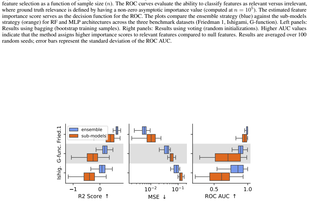
- The theory predicts that the accuracy gain carries over to feature selection: lower estimation error translates into higher ROC AUC for distinguishing relevant from irrelevant features, which the experiments confirm.
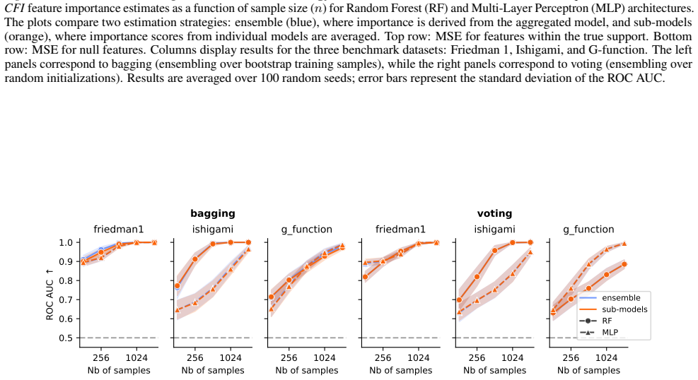
- For CFI, the two strategies are nearly equivalent, so the choice of aggregation matters mainly for risk-difference measures like LOCO and SAGE.
- The framework formalizes stability and the Rashomon effect: sampling-driven instability maps to estimation error and algorithmic stochasticity maps to optimization error, giving measurable meaning to these concepts.
Reading between the lines
- Editorial inference: because the core mechanism is excess-risk reduction, any intervention that lowers E—better hyperparameters, more training data, or distillation—should also sharpen LOCO/SAGE importance, not just ensembling.
- Editorial inference: the same bias-dominant logic likely extends to other risk-difference importance measures beyond LOCO and SAGE; testing it on a method like knockoff-based importance would be a natural check.
- Editorial inference: the UK Biobank results suggest that ensemble-based importance can recover known biomarkers with tighter error bars, but a replication on an independent proteomic cohort would test whether the rankings transfer across populations.
Editorial analysis
A structured set of objections, weighed in public.
Referee Report
Summary. The paper studies whether, for risk-based feature importance measures (LOCO, SAGE, CFI), one should compute importance on an ensemble predictor or average the importances of individual sub-models. The authors derive an error decomposition (Prop. 4.3, Thm. 4.6, Thm. 4.10) in which, under assumptions weaker than the Donsker-type conditions of Williamson et al. (2023), the leading estimation error is the model's excess risk rather than the finite-test-set term. They argue that model-level ensembling reduces this leading term via Jensen's inequality, while importance-level ensembling does not, leading to the recommendation in Remark 4.5 and the quantitative claim in Prop. 4.7. Experiments on Friedman 1, G-function, Ishigami, and a UK Biobank proteomic BMI application compare the two strategies for MLP and random-forest models under bagging and voting, reporting lower MSE and higher ROC AUC for model-level ensembling on LOCO and SAGE, with little difference for CFI.
Significance. If the theoretical claims held in their stated generality, the paper would provide a practically important and somewhat counterintuitive design rule: contrary to prior work that aggregates importance distributions (Donnelly et al., 2023), feature importance should be measured on the ensembled predictor itself. The empirical evaluation is a real strength: three benchmarks, two model classes, bagging and voting, separate support/null feature analysis, 100 seeds, MSE and ROC AUC, and a large real-world proteomic application. The initial decomposition, Prop. 4.3 and Thm. 4.6, is a clean consequence of the standard risk decomposition under the stated weak assumptions. However, the sharpest quantitative statement (Prop. 4.7) is not established as written, and the central 'bias-dominant regime' assumption is not empirically verified. The paper is therefore best viewed as a promising framework with strong empirical support rather than a fully supported theoretical result.
major comments (3)
- [Proposition 4.7 / Appendix A.3] The main text states ψ_ens − ψ⋆ = (ψ_sub − ψ⋆)(ρ + (1−ρ)/B) + O_P(n^{−1/2}), but the proof in Appendix A.3 concludes Δ_ens = Δ_sub · (1 + (1−ρ)/B) + O_P(n^{−1/2}). These factors agree only at ρ = 1; for ρ = 0 they are 1/B and 1 + 1/B, respectively. The proof also cancels bias terms using only the full-model equality Bias(f_ens)² = Bias(f_b)². For LOCO, the analogous equality for the restricted models, Bias(f_ens^{−j})² = Bias(f_b^{−j})², is neither stated nor proven. The Hastie variance formula further requires identical variances and pairwise correlation for both the full and restricted models. Without these conditions, Proposition 4.7 is not established. Please restate the proposition with explicit assumptions and correct the factor.
- [Remark 4.5 / Figure 3] The recommendation to prefer model-level ensembling is explicitly conditional on the 'bias-dominant regime' where the excess risk E converges slower than n^{−1/2}. The paper cites asymptotic class-level results (Bach 2024; Biau & Scornet 2016) to argue that modern models are in this regime, but these results do not establish that the specific MLP/RF fits on Friedman 1, G-function, and Ishigami at n = 256–2048 satisfy the condition. Figure 3 decomposes the MSE of importance estimates into squared bias and variance, but this is not a measurement of E relative to the O_P(n^{−1/2}) floor: the plotted bias already reflects the effect of ensembling on the importance estimate. If E is actually O_P(n^{−1/2}) or faster on these benchmarks, the test-set term A and remainder r_n can dominate, and the variance reduction from averaging sub-model importances may outweigh the bias reduction from ensemb
- [Section 4.1 / Appendix A.3] The definition of the restricted model for the ensemble strategy is not made precise enough for the comparison to be airtight. In Theorem 4.6, f_{θ,D_n}^{−j} is a model refitted without feature j. For ψ(f_ens, j), one needs R(f_ens^{−j}) − R(f_ens), but how is f_ens^{−j} constructed? If it is defined as the average of per-bootstrap restricted models, the linearity argument in Prop. 4.7 is plausible; if it is a single refitted model, it is not. The proof in Appendix A.3 silently assumes a relationship between f_ens^{−j} and {f_b^{−j}} that is never stated. Since the entire comparison between 'ensemble' and 'sub-models' hinges on this construction, please define it explicitly and verify the proof against the definition.
minor comments (4)
- [Appendix A.1, Eq. (8)] The decomposition in the proof of Prop. 4.3 writes R_n(f_{θ,D_n}) − R(f⋆) = A − E − r_n, but the correct expansion is A + E + r_n. The final result is correct, but the displayed sign errors should be fixed.
- [Appendix A.3] In the proof of Prop. 4.7, the displayed derivation contains sign errors: Δ_ens should be E(f_ens^{−j}) − E(f_ens) + O_P(n^{−1/2}), not with a plus sign. There is also a typo in the final line, where 'Δ_ens = Δ_sub · ...' is written as 'Δ_sub = Δ_sub · ...'.
- [Section 4.3 / Appendix C] The CFI error expression relies on Proposition 3.4 of Paillard et al. (2025), whose exact conditions are not restated in this paper. Since this external result is load-bearing for the CFI comparison, please state its assumptions or provide a self-contained derivation.
- [Appendix B, captions of Figures 11–12] The captions for the CFI MSE plots state 'error bars represent the standard deviation of the ROC AUC', which appears to be a copy-paste error; these figures show MSE, not ROC AUC.
Circularity Check
No significant circularity: the error decomposition and ensemble comparison rest on external results, and no fitted value is presented as a prediction.
full rationale
The derivation chain is not circular. Proposition 4.3 is obtained from the Williamson et al. (2023) decomposition, Kennedy's Lemma 1, and the CLT; Theorem 4.6 is a direct two-model application; Remark 4.5 follows from Jensen's inequality. No parameter is fitted and then renamed as a prediction; the MSE/ROC benchmarks use an independently computed asymptotic ground truth. The only overlapping-author citation is Proposition 3.4 of Paillard et al. (2025), used in Appendix C.1 to analyze the CFI contrast case; it is a published, externally falsifiable prior result, is not the basis of the central LOCO/SAGE claims, and is corroborated by the paper's own CFI experiments. I therefore do not count it as load-bearing circularity. The main-text Proposition 4.7 and its appendix proof do contain a rigor problem: the proof assumes (without stating) that the squared biases of the restricted and full models cancel, and the appendix ends with a factor 1+(1−ρ)/B while the main text states ρ+(1−ρ)/B. These are correctness/consistency concerns, not reductions of the conclusion to the inputs, so they do not raise the circularity score.
Assumptions & free parameters
free parameters (3)
- Asymptotic ground-truth sample size (n=10^5) =
10^5
- UK Biobank univariate pre-selection (top-50 proteins) =
50 features retained from 2,922
- Output correlation ρ (Prop 4.7) =
not estimated in experiments
assumptions (8)
- domain assumption Assumption 4.1: loss consistency — ||L(f_{θ,D_n}) − L(f⋆)||₂ = o_P(1)
- domain assumption Assumption 4.2: finite variance of the loss at f⋆
- domain assumption Assumption 4.8: support positivity — X has density bounded above and below on [0,1]^p
- domain assumption Assumption 4.9: K-Lipschitz loss
- domain assumption Bias-dominant regime: excess risk E converges slower than n^{−1/2} for expressive models
- ad hoc to paper Equal squared biases of restricted and full models: Bias(f̂^{-j})² = Bias(f̂)², with shared correlation ρ
- standard math Kennedy (2024) Lemma 1 bound on the cross-fit remainder
- standard math Variance-reduction formula Var(f̂_ens) = (ρ + (1−ρ)/B) Var(f̂) (Hastie et al. 2009)
Cite this review
Pith. "Pith review of Aggregate Models, Not Explanations: Improving Feature Importance Estimation." pith.science (2026). https://pith.science/paper/K5CNSJRO
@misc{pith2026260211760,
  author       = {Pith},
  title        = {Pith review of: Aggregate Models, Not Explanations: Improving Feature Importance Estimation},
  year         = {2026},
  howpublished = {\url{https://pith.science/paper/K5CNSJRO}},
  note         = {Machine review of arXiv:2602.11760}
}
read the original abstract
Feature-importance methods show promise in transforming machine learning models from predictive engines into tools for scientific discovery. However, due to data sampling and algorithmic stochasticity, expressive models can be unstable, leading to inaccurate variable importance estimates and undermining their utility in critical biomedical applications. Although ensembling offers a solution, deciding whether to explain a single ensemble model or aggregate individual model explanations is difficult due to the nonlinearity of importance measures and remains largely understudied. Our theoretical analysis, developed under assumptions accommodating complex state-of-the-art ML models, reveals that this choice is primarily driven by the model's excess risk. In contrast to prior literature, we show that ensembling at the model level provides more accurate variable-importance estimates, particularly for expressive models, by reducing this leading error term. We validate these findings on classical benchmarks and a large-scale proteomic study from the UK Biobank.
Figures


Figures from the paper (10 more)





Reference graph
Works this paper leans on
- [1]
-
[2]
14 Submission and Formatting Instructions for ICML 2026 (7) Conclusion.We conclude that ˆvf (S)−v f⋆ (S) =E h L E[ ˆf(X −S)|X S], y i −E L E[f⋆(X −S)|X S], y | {z } E S +Op(n−1/2)
For the first term, we use the Lipschitz assumption and the CLT to have that B1 ≤KE h ˆf S cal(x)−E[ ˆf(X −S)|X S] i =O p(n−1/2). 14 Submission and Formatting Instructions for ICML 2026 (7) Conclusion.We conclude that ˆvf (S)−v f⋆ (S) =E h L E[ ˆf(X −S)|X S], y i −E L E[f⋆(X −S)|X S], y | {z } E S +Op(n−1/2). Similarly, we have ˆvf (S∪ {j})−vf⋆ (S∪ {j}) =...
2026
-
[5]
We report the mean ROC AUC and its standard deviation across 100 random seeds
is strictly positive; this criterion captures both the Markov blanket (for LOCO) and all functionally linked features (for SAGE). We report the mean ROC AUC and its standard deviation across 100 random seeds. The extended results, presented in Figure 8 (LOCO) and Figure 9 (SAGE), compare theensemble 15 Submission and Formatting Instructions for ICML 2026 ...
2026
-
[8]
andSAGE(Figure 7 and Figure 9). Furthermore, these findings suggest that the error associated with estimating the conditional distribution—denoted as OP ||X π(j|−j) ⋆ −X π(j|−j) n ||2 2 —is not the limiting factor in practice. This aligns with the “Model-X” assumption (Candes et al., 2018), which posits that modeling the relationships among covariates (i....
2018
-
[9]
Under the mean squared error (MSE) loss, the trueCFIis defined as: ψcfi(j) =E y−f(X π(j|−j) ) 2 −E h (y−f(X)) 2 i (12) In practice, the conditional distribution P(X j|X −j) is unknown and must be estimated from data. To characterize the impact of this estimation, we denoteX π(j|−j) n as the random variable sampled from the estimated conditional distributi...
2025
-
[22]
org/10.1007/978-3-031-63797-1_22
URL http://dx.doi. org/10.1007/978-3-031-63797-1_22. Fisher, A., Rudin, C., and Dominici, F. All models are wrong, but many are useful: Learning a variable’s impor- tance by studying an entire class of prediction models simultaneously.Journal of Machine Learning Research, 20(177):1–81,
-
[2001]
A princi- pled approach for comparing variable importance.arXiv preprint arXiv:2507.17306,
Reyero-Lobo, A., Neuvial, P., and Thirion, B. A princi- pled approach for comparing variable importance.arXiv preprint arXiv:2507.17306,
-
[2010]
URL http: //www.jstor.org/stable/41058949
ISSN 08834237. URL http: //www.jstor.org/stable/41058949. Sudlow, C., Gallacher, J., Allen, N., Beral, V ., Burton, P., Danesh, J., Downey, P., Elliott, P., Green, J., Landray, M., et al. Uk biobank: an open access resource for identifying the causes of a wide range of complex diseases of middle and old age.PLoS medicine, 12(3):e1001779,
Show all 10 references
-
[2023]
Proofs A.1
10 Submission and Formatting Instructions for ICML 2026 A. Proofs A.1. Proof of Proposition 4.3 Assumption:Loss consistencyf θ,Dnis a minimizer of the risk:||L(f θ,Dn (X), Y)− L(f⋆(X), Y)||2 =o P (1) Assumption:Finite variance of the lossThe loss function, evaluated at the ris...
2026
-
[2025]
Sensitivity analysis in practice: a guide to assessing sci- entific models, volume
9 Submission and Formatting Instructions for ICML 2026 Saltelli, A., Tarantola, S., Campolongo, F., Ratto, M., et al. Sensitivity analysis in practice: a guide to assessing sci- entific models, volume
2026
Reviewed August 3, 2026 · model on record in the stance chip above.
Discussion (0). Sign in to comment.