REVIEW 3 major objections 5 minor 41 references
NeuPDE: Neural Network Based Ordinary and Partial Differential Equations for Modeling Time-Dependent Data
T0 review · 3 major / 5 minor · reviewed 2026-08-14 · deepseek-v4-flash
Pith's one-line read NeuPDE recovers governing ODEs and PDEs from trajectory data by pairing a monomial dictionary with a shallow network.
desk verdict Plausible architecture, but the only PDE-discovery experiment is undermined by a training/test initial-condition mismatch that leaves the central claim unproven. read the letter →
The pith
A machine-rendered reading of the paper's core claim, the machinery that carries it, and where it could break.
The reading
What carries the argument
The load-bearing object is the dictionary-plus-MLP operator $F(D(\cdot),\theta)$, where $D$ is the matrix of all monomials $t^k x_1^{\ell_1}\cdots x_d^{\ell_d}$ with $0<k+\sum_i \ell_i\le p$, plus, for PDEs, the same construction over $t$, $x$, $u$, and finite-difference approximations of spatial derivatives. $F$ is a two-layer MLP with a smooth activation; the ODE/PDE constraint $\dot{x}=F(D(N(x)),\theta)$ is enforced by integrating the equation with a Runge-Kutta scheme inside the loss, and temporal mini-batches of short trajectories are used with Adam. In the image-classification variant, the same idea becomes a semi-discrete PDE whose $3\times 3$ convolution kernels lie in the span of six finite-difference kernels (identity, $D_x$, $D_y$, $D_{xx}$, $D_{xy}$, $D_{yy}$), so each layer is an explicit differential operator rather than a free kernel.
What would settle it
Train the Burgers model on the paper's sine-in-x initial data and evaluate on sine-in-y initial data over a horizon longer than $T=0.015$, comparing the prediction error against the error of a baseline that returns the nearest training snapshot. If the NeuPDE error is not clearly smaller, or if it grows at the same rate as the training-data spread, the model has memorized trajectories rather than inferred the differential operator. The paper's reported test MSE of 3.6, versus training MSE of 0.005, is exactly the quantity to watch, normalized by the test data variance.
Extended reading notes
Core claim
The central claim is that the forcing function of a neural ODE/PDE should not be a generic MLP on raw inputs, but an MLP applied to a dictionary of the time variable, state components, and, in the PDE case, finite-difference approximations of spatial derivatives. In the paper's notation the model is $\dot{x}=F(D(N(x)),\theta)$, with $F(z,\theta)=A_2\sigma(A_1 z+b_1)+b_2$; training minimizes trajectory misfit plus an $\ell^1$ weight penalty and an $\ell^2$ penalty on the time derivative, while the state sequence is constrained to be the output of a Runge-Kutta solver. The authors demonstrate that this parameterization identifies accurate dynamics where sparse polynomial methods miss a time-dependent term, improves an eight-mode DMD reduced model of the von Kármán vortex sheet, and, when convolution kernels are restricted to linear combinations of finite-difference operators, matches or improves image-classification accuracy with fewer parameters than the baselines.
Load-bearing premise
The learned differential operator is assumed to transfer to initial conditions outside the training set, so the model must have inferred the dynamics rather than memorized the particular trajectories it was trained on.
Editorial extensions
If this is right
- Learned models are continuous differential equations, so after training they can be queried and integrated at arbitrary time resolutions, not only at the observed time stamps.
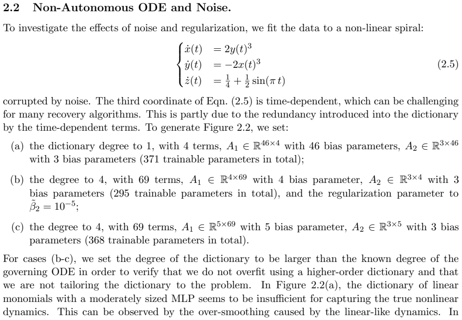
- In the noisy spiral example, the method recovered the time-dependent z-dynamics that SINDy and LASSO failed to recover, indicating the dictionary-MLP parameterization can handle time-dependent terms and noise better than fixed sparse dictionaries.
- The low-rank fluid example shows a learned nonlinear closure term can improve an eight-mode DMD reduced model, cutting terminal relative $L^2$ error from 0.060 to 0.049; more modes would make DMD accurate, but the closure provides an alternative.
- On MNIST, restricting kernels to finite-difference operators preserves 0.51% error while reducing parameters from ODE-Net's 0.22M to 0.18M; on Fashion MNIST, 0.38M parameters outperform ResNet18's 2.78M parameters at 7.6% versus 8.0% error.
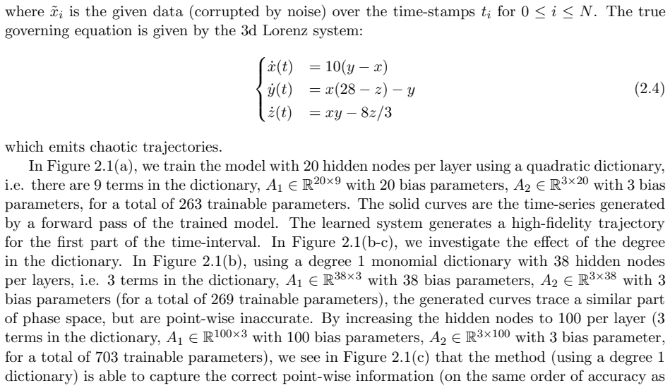
- Using a quadratic dictionary for Lorenz, 263 parameters track the trajectory as well as a degree-one dictionary with 703 parameters, so the dictionary level is a direct control on model capacity.
Reading between the lines
- The paper leaves dictionary degree and MLP width as hand-set hyperparameters; a natural next step is to add sparsity over dictionary entries so the method selects its own monomials.
- The paper tests fixed-horizon errors only; feeding the model's own predictions back as initial conditions over many cycles would reveal whether the learned operator is stable under iteration.
- The finite-difference kernel basis suggests a broader design principle: constraining convolution layers to learned linear combinations of differential operators may transfer parameter savings to larger image and video tasks.
Signed reviews
Editorial analysis
A structured set of objections, weighed in public.
Referee Report
Summary. The manuscript proposes NeuPDE, a framework that models time-dependent data by learning the right-hand side of an ordinary or partial differential equation. The unknown forcing term is parameterized as a shallow MLP applied to a monomial dictionary of the state variables (and, for PDEs, finite-difference derivative approximations), and the model is trained by fitting trajectories produced by a numerical integrator to observed data, using a regularized loss and a discretize-then-optimize backpropagation approach. The paper demonstrates the method on the Lorenz system, a noisy non-autonomous spiral ODE, a low-rank von Kármán vortex sheet, a 2D Burgers equation, and image classification on MNIST and Fashion-MNIST. The central claims are that NeuPDE can extract accurate governing ODE/PDE models, improve reduced-order modeling, and reduce the parameter cost relative to standard deep networks.
Significance. If established, the hybrid dictionary-MLP parameterization is a worthwhile contribution: it connects sparse dictionary-based equation discovery with neural network flexibility, and the finite-difference kernel constraint for image classification offers a parameter-efficient alternative to standard convolutional layers. The paper is clearly written and the formulation is easy to follow. However, the central PDE-discovery claim rests on a single Burgers experiment whose training and test initial conditions are not aligned, and the baseline comparisons are sparse. The image-classification results, while empirically plausible, are parameter-count comparisons rather than demonstrations of equation discovery. The manuscript would be strengthened materially by a corrected or extended PDE experiment and by quantitative evaluations of the ODE examples.
major comments (3)
- [Sec. 3.1, Eq. (3.3)] The Burgers experiment does not support the claim that NeuPDE identifies a governing PDE. All five training trajectories use a sine-in-x initial condition; for the 2D Burgers equation, such initial data has u_y and u_yy identically zero along the entire trajectory (up to the small added noise). Consequently, the dictionary channels containing y-derivatives are unexcited during training, the gradient of the loss provides essentially no information about their weights, and those weights remain unconstrained. The test initial condition, sine-in-y, activates exactly those channels, and the reported train/test MSE of 0.005/3.6 is the expected signature of a fit to the x-dependent training manifold rather than of a discovered differential operator. To support the PDE-discovery claim, the authors must either train on initial conditions that excite all derivative directions, or demonstrate generalization on multiple genuinely unseen initial conditions from the same PDE, ideally also inspecting the learned RHS against the true Burgers operator.
- [Sec. 2.3] The comparisons to SINDy and LASSO are shown only for the non-autonomous noisy spiral of Section 2.2, and SINDy fails on that example while LASSO fails in the z-component. No data-discovery baseline is reported for the Burgers PDE experiment, even though the abstract states a comparison to "other data-discovery methods" and the PDE case is the central novelty. Please add a PDE-discovery baseline (for example, PDE-FIND-style sparse regression or a dictionary-based method) to the Burgers example, and also provide quantitative comparisons for the autonomous Lorenz ODE example so that the reader can judge the performance relative to standard sparse identification.
- [Sec. 2.1, Fig. 2.1] The Lorenz experiment is evaluated only qualitatively, with the statement that the learned system generates a "high-fidelity trajectory for the first part of the time-interval." No quantitative error, prediction horizon, or learned coefficients are reported. For a chaotic system, short-horizon agreement can be achieved by models that do not identify the true governing equations, so this demonstration is weak evidence for the method's discovery capability. Please report the normalized prediction error as a function of lead time, the length of the accurate prediction interval, and, if possible, a comparison of the learned dynamics with the true Lorenz system in phase-space or via coefficient recovery.
minor comments (5)
- [Sec. 2, definition of ELU] The definition of σ_ELU appears to be inverted: the standard ELU is x for x >= 0 and e^x - 1 for x < 0, whereas the text states e^x - 1 for x >= 0 and x for x < 0. Please correct this, as it affects the implementation.
- [Sec. 2, text] There is a typo: "we purpose a different parameterization" should read "we propose a different parameterization."
- [Sec. 3.2, text] The word "semi-discete" should be "semi-discrete" in the description of the PDE block.
- [Eq. (2.1) and Eq. (2.2)] The relationship between the continuous-time derivative regularizer in Eq. (2.1) and the finite-difference sum in Eq. (2.2) is stated only as "β2 rescaled by the time-step." Please spell out the rescaling formula so that the discretization is unambiguous.
- [Fig. 3.1 caption] The caption for Figure 3.1 says "(a) Training data. (b) Learned surface, test data," while the text says the learned solution is plotted on both training and test sets. Please make the caption consistent with the text and clarify which quantity is shown at the terminal time.
Circularity Check
No circularity found: NeuPDE is a data-fitting architecture whose predictions are evaluated on held-out time stamps and initial conditions; the self-citations are background, and the Burgers train/test gap is a generalization concern, not a circular dependency.
full rationale
The paper's derivation chain is an empirical fitting procedure: it parameterizes the unknown ODE/PDE right-hand side as F(D(...),theta) with a monomial dictionary and an MLP, then minimizes a data-misfit loss (Eqs. 2.1, 2.2, 2.3, 3.3) over the parameters. The learned model is then used to generate trajectories from initial data, and these are compared with held-out data. Nothing in the construction defines the target output as an input to the model: the dictionary terms are candidate features, the finite-difference kernels are fixed numerical derivative approximations, and the train/test splits are genuine. Baselines (SINDy, LASSO, DMD, RNN, ODE-Net) are external. The paper includes several self-citations (e.g., refs. 32-35, 40-41), but they are used for background on sparse dictionary methods, for convergence theory of the SINDy baseline, and for ResNet stability; none is invoked as the justification that NeuPDE's model is correct or unique. The Burgers experiment in Sec. 3.1 reports train MSE 0.005 and test MSE 3.6 when the test initial condition is sine-in-y rather than sine-in-x; this is evidence that the fitted model may not have learned a generalizable differential operator, and it is a correctness/validation concern rather than a circular argument. Every claimed prediction is produced by forward integration of the trained right-hand side, not by a quantity that was fitted into the loss. Therefore the circularity score is 0.
Assumptions & free parameters
free parameters (3)
- Dictionary degree p =
1, 2, or 4 depending on experiment
- Hidden units per layer =
20, 38, 50, 64, 100, 128 depending on experiment
- Regularization weights beta1 and beta2 =
beta1=1e-4, beta2=1e-5 (claimed no tuning)
assumptions (5)
- domain assumption The time-series data is governed by a first-order ODE of the form dx/dt = f(t,x).
- domain assumption For spatio-temporal data, the evolution is first-order in time and can be written as u_t = G(t,x,u,Du,...).
- domain assumption The unknown right-hand side f or G can be accurately approximated by an MLP over the monomial dictionary.
- domain assumption The finite-difference approximations to spatial derivatives are sufficiently accurate at the available grid resolution.
- standard math The numerical ODE solver (Runge-Kutta) advances the state accurately enough, and backpropagation through the solver is stable.
Cite this review
Pith. "Pith review of NeuPDE: Neural Network Based Ordinary and Partial Differential Equations for Modeling Time-Dependent Data." pith.science (2026). https://pith.science/paper/K6KHZPNR
@misc{pith2026190803190,
  author       = {Pith},
  title        = {Pith review of: NeuPDE: Neural Network Based Ordinary and Partial Differential Equations for Modeling Time-Dependent Data},
  year         = {2026},
  howpublished = {\url{https://pith.science/paper/K6KHZPNR}},
  note         = {Machine review of arXiv:1908.03190}
}
read the original abstract
We propose a neural network based approach for extracting models from dynamic data using ordinary and partial differential equations. In particular, given a time-series or spatio-temporal dataset, we seek to identify an accurate governing system which respects the intrinsic differential structure. The unknown governing model is parameterized by using both (shallow) multilayer perceptrons and nonlinear differential terms, in order to incorporate relevant correlations between spatio-temporal samples. We demonstrate the approach on several examples where the data is sampled from various dynamical systems and give a comparison to recurrent networks and other data-discovery methods. In addition, we show that for MNIST and Fashion MNIST, our approach lowers the parameter cost as compared to other deep neural networks.
Figures


Figures from the paper (4 more)


Reference graph
Works this paper leans on
-
[1]
https://github.com/zalandoresearch/fashion-mnist
Fashion MNIST Dataset. https://github.com/zalandoresearch/fashion-mnist
-
[2]
https://github.com/kefth/fashion-mnist
Fashion MNIST ResNet18. https://github.com/kefth/fashion-mnist
-
[3]
https://github.com/heitorrapela/fashion-mnist-mlp
MLP for Fashion MNIST. https://github.com/heitorrapela/fashion-mnist-mlp
-
[4]
Discovering governing equations from data by sparse identification of nonlinear dynamical systems
Steven L Brunton, Joshua L Proctor, and J Nathan Kutz. Discovering governing equations from data by sparse identification of nonlinear dynamical systems. Proceedings of the National Academy of Sciences, 113(15):3932–3937, 2016
work page 2016
-
[5]
Neural ordinary differential equations
Tian Qi Chen, Yulia Rubanova, Jesse Bettencourt, and David K Duvenaud. Neural ordinary differential equations. In Advances in Neural Information Processing Systems , pages 6571– 6583, 2018
work page 2018
-
[6]
Deep learning for physical pro- cesses: Incorporating prior scientific knowledge
Emmanuel de Bezenac, Arthur Pajot, and Patrick Gallinari. Deep learning for physical pro- cesses: Incorporating prior scientific knowledge. arXiv preprint arXiv:1711.07970 , 2017
arXiv 2017
-
[7]
A proposal on machine learning via dynamical systems
Weinan E. A proposal on machine learning via dynamical systems. Communications in Math- ematics and Statistics , 5(1):1–11, 2017. 14
work page 2017
-
[8]
ANODE: Unconditionally accurate memory- efficient gradients for neural ODEs
Amir Gholami, Kurt Keutzer, and George Biros. ANODE: Unconditionally accurate memory- efficient gradients for neural ODEs. arXiv preprint arXiv:1902.10298 , 2019
arXiv 1902
Show all 41 references
-
[9]
Learning, invariance, and generalization in high-order neural networks
C Lee Giles and Tom Maxwell. Learning, invariance, and generalization in high-order neural networks. Applied optics, 26(23):4972–4978, 1987
1987
-
[10]
Stable architectures for deep neural networks
Eldad Haber and Lars Ruthotto. Stable architectures for deep neural networks. Inverse Problems, 34(1):014004, January 2017
2017
-
[11]
Deep residual learning for image recognition
Kaiming He, Xiangyu Zhang, Shaoqing Ren, and Jian Sun. Deep residual learning for image recognition. ArXiv e-prints, December 2015
2015
-
[12]
Identity mappings in deep residual networks
Kaiming He, Xiangyu Zhang, Shaoqing Ren, and Jian Sun. Identity mappings in deep residual networks. ArXiv e-prints, March 2016
2016
-
[13]
Turbulence, coherent structures, dynamical systems and symmetry
Philip Holmes, John L Lumley, Gahl Berkooz, and Clarence W Rowley. Turbulence, coherent structures, dynamical systems and symmetry . Cambridge university press, 2012
2012
-
[14]
Weinberger
Gao Huang, Zhuang Liu, Laurens van der Maaten, and Kilian Q. Weinberger. Densely con- nected convolutional networks. ArXiv e-prints, August 2016
2016
-
[15]
Batch normalization: Accelerating deep network training by reducing internal covariate shift
Sergey Ioffe and Christian Szegedy. Batch normalization: Accelerating deep network training by reducing internal covariate shift. arXiv preprint arXiv:1502.03167 , 2015
2015 arXiv
-
[16]
Adam: A method for stochastic optimization
Diederik P Kingma and Jimmy Ba. Adam: A method for stochastic optimization. arXiv preprint arXiv:1412.6980, 2014
2014 arXiv
-
[17]
Nathan Kutz, Steven L
J. Nathan Kutz, Steven L. Brunton, Bingni W. Brunton, and Joshua L. Proctor. Dynamic Mode Decomposition: Data-driven modeling, Equation-free modeling of Complex systems . SIAM, 2016
2016
-
[18]
Dynamic mode decomposition: data-driven modeling of complex systems
J Nathan Kutz, Steven L Brunton, Bingni W Brunton, and Joshua L Proctor. Dynamic mode decomposition: data-driven modeling of complex systems . SIAM, 2016
2016
-
[19]
FractalNet: Ultra-deep neural networks without residuals
Gustav Larsson, Michael Maire, and Gregory Shakhnarovich. FractalNet: Ultra-deep neural networks without residuals. ArXiv e-prints, May 2016
2016
-
[20]
Gradient-based learning applied to document recognition
Yann LeCun, L´ eon Bottou, Yoshua Bengio, Patrick Haffner, et al. Gradient-based learning applied to document recognition. Proceedings of the IEEE, 86(11):2278–2324, 1998
1998
-
[21]
Pde-net 2.0: Learning PDEs from data with a numeric-symbolic hybrid deep network
Zichao Long, Yiping Lu, and Bin Dong. Pde-net 2.0: Learning PDEs from data with a numeric-symbolic hybrid deep network. arXiv preprint arXiv:1812.04426 , 2018
2018 arXiv
-
[22]
Pde-net: Learning PDEs from data
Zichao Long, Yiping Lu, Xianzhong Ma, and Bin Dong. Pde-net: Learning PDEs from data. arXiv preprint arXiv:1710.09668 , 2017
2017 arXiv
-
[23]
Beyond finite layer neural net- works: Bridging deep architectures and numerical differential equations
Yiping Lu, Aoxiao Zhong, Quanzheng Li, and Bin Dong. Beyond finite layer neural net- works: Bridging deep architectures and numerical differential equations. arXiv preprint arXiv:1710.10121, 2017. 15
2017 arXiv
-
[24]
Autograd: Reverse-mode differen- tiation of native python
Dougal Maclaurin, David Duvenaud, and Ryan P Adams. Autograd: Reverse-mode differen- tiation of native python. In ICML workshop on Automatic Machine Learning , 2015
2015
-
[25]
Data driven governing equations approximation using deep neural networks
Tong Qin, Kailiang Wu, and Dongbin Xiu. Data driven governing equations approximation using deep neural networks. arXiv preprint arXiv:1811.05537 , 2018
2018 arXiv
-
[26]
Hidden physics models: Machine learning of nonlinear partial differential equations
Maziar Raissi and George Em Karniadakis. Hidden physics models: Machine learning of nonlinear partial differential equations. Journal of Computational Physics , 357:125–141, 2018
2018
-
[27]
Machine learning of linear differential equations using Gaussian processes
Maziar Raissi, Paris Perdikaris, and George Em Karniadakis. Machine learning of linear differential equations using Gaussian processes. Journal of Computational Physics , 348:683– 693, 2017
2017
-
[28]
Physics informed deep learning (part ii): Data-driven discovery of nonlinear partial differential equations
Maziar Raissi, Paris Perdikaris, and George Em Karniadakis. Physics informed deep learning (part ii): Data-driven discovery of nonlinear partial differential equations. arXiv preprint arXiv:1711.10566, 2017
2017 arXiv
-
[29]
Data-driven discovery of partial differential equations
Samuel H Rudy, Steven L Brunton, Joshua L Proctor, and J Nathan Kutz. Data-driven discovery of partial differential equations. Science Advances, 3(4):e1602614, 2017
2017
-
[30]
Deep neural networks motivated by partial differential equa- tions
Lars Ruthotto and Eldad Haber. Deep neural networks motivated by partial differential equa- tions. ArXiv e-prints, April 2018
2018
-
[31]
Weight normalization: A simple reparameterization to accelerate training of deep neural networks
Tim Salimans and Durk P Kingma. Weight normalization: A simple reparameterization to accelerate training of deep neural networks. In Advances in Neural Information Processing Systems, pages 901–909, 2016
2016
-
[32]
Learning partial differential equations via data discovery and sparse opti- mization
Hayden Schaeffer. Learning partial differential equations via data discovery and sparse opti- mization. Proceedings of the Royal Society A: Mathematical, Physical and Engineering Sci- ences, 473(2197):20160446, 2017
2017
-
[33]
Sparse model selection via integral terms
Hayden Schaeffer and Scott G McCalla. Sparse model selection via integral terms. Physical Review E, 96(2):023302, 2017
2017
-
[34]
Learning dynamical systems and bifurcation via group sparsity
Hayden Schaeffer, Giang Tran, and Rachel Ward. Learning dynamical systems and bifurcation via group sparsity. arXiv preprint arXiv:1709.01558 , 2017
2017 arXiv
-
[35]
Extracting sparse high-dimensional dynamics from limited data
Hayden Schaeffer, Giang Tran, and Rachel Ward. Extracting sparse high-dimensional dynamics from limited data. SIAM Journal on Applied Mathematics , 78(6):3279–3295, 2018
2018
-
[36]
Dynamic Mode Decomposition of numerical and experi- mental data
Peter Schmid and Joern Sesterhenn. Dynamic Mode Decomposition of numerical and experi- mental data. Bulletin of the American Physical Society , 53, 2008
2008
-
[37]
Dynamic mode decomposition of numerical and experimental data
Peter J Schmid. Dynamic mode decomposition of numerical and experimental data. Journal of fluid mechanics , 656:5–28, 2010
2010
-
[38]
The pi-sigma network: An efficient higher-order neural network for pattern classification and function approximation
Yoan Shin and Joydeep Ghosh. The pi-sigma network: An efficient higher-order neural network for pattern classification and function approximation. In IJCNN-91-Seattle International Joint Conference on Neural Networks , volume 1, pages 13–18. IEEE, 1991. 16
1991
-
[39]
Exact recovery of chaotic systems from highly corrupted data
Giang Tran and Rachel Ward. Exact recovery of chaotic systems from highly corrupted data. Multiscale Modeling & Simulation , 15(3):1108–1129, 2017
2017
-
[40]
Forward stability of resnet and its variants
Linan Zhang and Hayden Schaeffer. Forward stability of resnet and its variants. arXiv preprint arXiv:1811.09885, 2018
2018 arXiv
-
[41]
On the convergence of the sindy algorithm
Linan Zhang and Hayden Schaeffer. On the convergence of the sindy algorithm. Multiscale Modeling & Simulation , 17(3):948–972, 2019. 17 A Derivation of Adjoint Equations Let θ be the vector of learnable parameters (that parameterizes the unknown function g, which embeds all net...
2019
Reviewed August 14, 2026 · model on record in the stance chip above.
Discussion (0). Continue with ORCID to comment.