REVIEW 4 major objections 4 minor 40 references
A Generative Framework for the Creation of Multi-Attribute Geographically-Explicit Synthetic Population
T0 review · 4 major / 4 minor · reviewed 2026-08-15 · deepseek-v4-flash
Pith's one-line read A two-stage diffusion framework generates a 332-million-person synthetic U.S. population while reconstructing regional five-attribute joint distributions more accurately than IPF, combinatorial optimization, or a one-shot diffusion model.
desk verdict A substantial national synthetic population dataset with a two-stage diffusion model, but the headline held-out validation is weakened by tuning the coarse state size on the test region. read the letter →
The pith
A machine-rendered reading of the paper's core claim, the machinery that carries it, and where it could break.
The reading
What carries the argument
The load-bearing mechanism is the two-stage coarse-to-fine diffusion factorization, expressed as $\hat{p}_k = \hat{p}^{c}_{g(k)} \hat{p}^{i}_{k|g(k)}$. Stage 1 denoises a 960-cell log-probability vector, conditioned on a learned encoding of the region's ACS marginals and its 235-dimensional spatial signature built from point-of-interest and commuting-flow data; Stage 2 denoises each within-coarse refinement vector, conditioned on the coarse group label and its Stage-1 probability. This hierarchical split is what lets the model learn region-level demographic structure before resolving fine-grained attribute combinations, and it is the design choice that distinguishes the framework from the one-stage diffusion baseline it beats.
What would settle it
Hold out a demographically unusual state, say one dominated by large university towns, and run the framework conditioned only on that state's ACS marginals and POI/LODES vector; if its predicted 3,000-cell joint distribution has a TVD no better than IPF, or if the Stage-2 refinement distributions are essentially flat and identical across PUMAs, the claim that the spatial signature carries the non-stationary co-occurrence signal would be contradicted.
Extended reading notes
Core claim
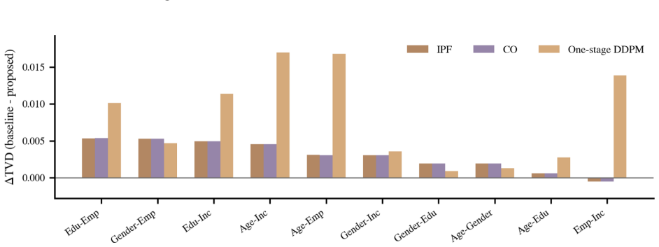
The central claim is that a five-attribute joint distribution for any region can be reconstructed as the product of a coarse distribution and within-coarse refinements, with both levels generated by diffusion. Stage 1 predicts a 960-cell coarse distribution from the region's aggregated marginals and its spatial signature; Stage 2 takes each coarse cell, together with its Stage-1 probability, and distributes that mass over the fine-grained combinations it contains, so the final probability of a fine combination $k$ is $\hat{p}_k = \hat{p}^{c}_{g(k)} \hat{p}^{i}_{k|g(k)}$. The framework trains on joint distributions estimated from PUMS for 2,462 PUMAs and at inference conditions only on ACS counts and the 235-dimensional POI/LODES vector, which is what lets it produce joint distributions for regions never seen in training. The authors' evidence for this is two-pronged: internally, the synthetic population's joint distributions overlap the PUMS targets to mean TVD 0.116; externally, Michigan's held-out PUMAs come in at mean TVD 0.119, below IPF, combinatorial optimization, and a one-stage DDPM, with the pairwise decomposition showing the gains concentrated in attribute pairs—education–employment, gender–employment, education–income, age–income—whose joint distributions are absent from the aggregate census tables. After sampling individuals from $\hat{p}$, Step 3 places homes and workplaces on the road network using tract-level ACS counts and commuting-flow data, preserving major residential and workplace patterns.
Load-bearing premise
The framework's generalization rests on the assumption that a region's five-attribute joint distribution can be predicted from its aggregated census marginals plus its 235-dimensional description of local businesses and commuting flows, so any co-occurrence pattern these inputs do not reveal cannot be recovered for a region outside the training set.
Editorial extensions
If this is right
- A region can be synthesized without its own microdata: only aggregated census marginals and the POI/LODES spatial vector are needed as conditions at inference, so the trained model applies across all 2,462 PUMAs.
- The released dataset gives agent-based models a national population of 332,387,543 individuals whose attributes co-occur according to region-specific PUMS evidence rather than a fixed heuristic.
- The TVD gains over IPF and CO appear exactly where aggregate tables are silent—education–income, age–income, education–employment, gender–employment—so the model is recovering latent socioeconomic dependencies.
- Because synthesis is one forward pass of a trained model rather than a per-region optimization, extending the population to a new state or region is cheaper than combinatorial approaches.
- The 960-cell coarse target lies on a stable accuracy plateau, so the hierarchical design keeps Stage 1 compact without sacrificing held-out joint-distribution accuracy.
Reading between the lines
- The coarse-to-fine factorization is not tied to five attributes; we would expect it to extend to household structure, race, or richer income brackets, provided the condition vectors are extended to carry the new co-occurrence signals.
- The sharpest unstated test of the mechanism is to hold out a demographically atypical region—a college town or retirement hub—and see whether the POI/LODES vector alone steers Stage 1 to the right part of the state space; we would expect gains to shrink where the spatial signature does not reflect the region's co-occurrence pattern.
- The Stage-2 refinement probabilities could be used as diagnostics: coarse cells whose within-coarse distributions vary most across PUMAs identify exactly which attribute combinations carry the spatial non-stationarity.
- A limit the paper itself acknowledges: ages are produced as groups rather than exact values, children under 18 receive no daytime locations because LODES only covers employed adults, and home/work placement is constrained by available road and commuting data—so the dataset's fine-grained mobility uses are bounded.
Signed reviews
Editorial analysis
A structured set of objections, weighed in public.
Referee Report
Summary. The paper proposes a hierarchical, two-stage diffusion-based framework for generating a five-attribute, geographically-explicit synthetic population for the entire United States. Stage 1 predicts a coarse joint distribution over grouped categories (K=960 combinations) from ACS marginal conditions and a 235-dimensional spatial representation built from POI and LODES data; Stage 2 refines each coarse cell into fine-grained combinations, yielding a 3,000-dimensional joint distribution per PUMA. Synthetic individuals are then sampled from these distributions and assigned home and work locations using tract-level ACS data, LODES flows, and road networks. The authors report low internal TVD on training PUMAs, small marginal discrepancies against ACS, and a held-out Michigan experiment in which their method achieves mean TVD 0.119 versus 0.12698 for IPF, 0.12697 for CO, and 0.14707 for a one-stage diffusion baseline. The main generalizability claim rests on this held-out comparison.
Significance. If the held-out generalization claim survives scrutiny, the framework would be a useful contribution to synthetic population generation: it directly targets region-specific joint distributions, uses openly available data, and ships both the generated dataset (OSF) and code (GitHub). The hierarchical coarse-to-fine diffusion design is a sensible way to reduce the difficulty of predicting a 3,000-dimensional target, and the internal validation is a useful descriptive check. However, the paper's central claim of improved held-out reconstruction is currently weakened by test-set hyperparameter selection and by the absence of uncertainty quantification on the headline comparison. The contribution is potentially significant for geo-simulation and agent-based modeling applications, but the evidence for generalization needs to be re-established with an unbiased evaluation protocol.
major comments (4)
- [Section A.2 and Section 3.2] The headline held-out result is compromised by test-set selection. Section A.2 states that candidate coarse state-space sizes K were evaluated 'using the held-out TVD metric across the 68 Michigan PUMAs' and that K=960 was chosen because it sits on the plateau in Figure S1. Michigan is therefore not an untouched test region: the global hyperparameter K was selected to optimize the exact quantity reported in Section 3.2. The plateau in Figure S1 may limit the resulting bias, but the reported 6.3% relative TVD reduction over IPF and CO cannot be treated as an independent estimate unless K is fixed using only training-state data, or unless the evaluation is repeated for every candidate K and all held-out states. Please add such an analysis and clearly report the model-selection procedure.
- [Section 3.2 and Table S1] The held-out comparison reports only point estimates of mean TVD (0.119 versus 0.12698 and 0.12697), while the internal validation reports a seed-level standard deviation of 0.01586 for a mean TVD of 0.11651. No confidence intervals, paired per-seed comparisons, or significance tests are given for the Michigan experiment. With a raw TVD difference of roughly 0.008 (Table S1), the claimed improvement over IPF and CO is not statistically supported as reported. Please report per-seed results for each baseline and method, and provide paired tests or bootstrap confidence intervals.
- [Section 3.2, IPF baseline] The IPF baseline appears to be specified in a way that may understate its performance. The text says IPF adjusts 'a fixed seed table, which represents the average joint distribution over training PUMAs,' rather than a seed derived from the held-out region's own PUMS sample, which is the standard practice for IPF-based population synthesis. This choice by construction limits the baseline's ability to capture regional co-occurrence patterns and may inflate the reported gain. Please re-run IPF with a locally representative seed (e.g., the Michigan PUMS joint distribution) or justify the fixed average seed as the only information allowed under the paper's data-access assumptions.
- [Section 2.4.1 and Table 4] The paper does not provide an ablation or quantitative test of whether the 235-dimensional spatial representation h actually improves reconstruction relative to using only the ACS marginal condition c. Since the spatial representation is a central component of the claimed ability to preserve spatial non-stationarity, please include an experiment that removes h (or replaces it with a simpler control) and report the effect on held-out TVD. Without this, the reader cannot tell whether the spatial representation is load-bearing for the reported results.
minor comments (4)
- [Section 2.5, Eq. (2)] In Equation 2, the symbol N_{r,k} is used before it is defined; please define all quantities before first use, including N_{t,a,v}, q(t|k), and N_{r,k}.
- [Section 2.4.2 and Table 4] The fine-grained age categories are inconsistent: Section 2.4.2 says Stage 2 refines the 18–34 coarse group into 18–24 and 25–34, while Table 4 lists age groups as [18,25) and [25,35). Please align the age boundaries across the main text and the data dictionary.
- [Section 3.2, Figure 3] The reference to Figure 3 is inconsistent: the text mentions 'Figure (a)' and 'Figure 3 (b)', while the caption describes panels (a) and (b). Please use consistent figure/panel references throughout.
- [Section A.1] The description of the 235-dimensional spatial representation is detailed but would benefit from a table summarizing the number of components per level; currently the counts (218 POI + 17 LODES = 235) require manual summation from the text.
Circularity Check
Michigan held-out result is selected on the same Michigan test set via the K sensitivity analysis, so the headline TVD gain is not an independent out-of-sample measurement.
-
fitted input called prediction
[Supplementary A.2 (Sensitivity to the Coarse Variable Combinations Size); Section 2.4.1 (Stage 1); Section 3.2 (Validation)]
"Under the same POI+LODES condition setting, we evaluate candidate values of K using the held-out TVD metric across the 68 Michigan PUMAs. ... We therefore use K= 960 as the default coarse state-space size, since it preserves plateau-level accuracy while keeping the Stage 1 prediction target more compact. ... Its mean TVD is 0.119, compared with 0.12698 for IPF, 0.12697 for CO, and 0.14707 for the one-stage DDPM baseline."
The Stage-1 coarse state-space size K is a global model hyperparameter. Section 2.4.1 states that K=960 is selected based on a sensitivity analysis, and Supplementary A.2 describes that analysis as evaluating candidate K values using the held-out TVD metric across the 68 Michigan PUMAs. The headline held-out result in Section 3.2 is then measured on exactly those 68 Michigan PUMAs. Michigan has therefore already influenced model configuration before serving as the test region; the reported mean TVD of 0.119 and the 6.3% reduction over IPF/CO are selected values, not an independent out-of-sample measurement. This is selection on the test set and can only bias the generalization estimate optimistically.
full rationale
The derivation chain is otherwise self-contained: the training target p is the PUMS empirical joint distribution, conditions c and h are independent census/spatial aggregates, and the diffusion models learn a mapping from conditions to targets. The hierarchical factorization in Eq. 1 (p_k = p_coarse_g(k) * p_inner_k|g(k)) is a decomposition of the target, not a hidden reuse of the output. Internal validation against the training target is in-sample fit, which is expected and not circular. The one circular step is the selection of K on the Michigan held-out TVD followed by reporting that same Michigan held-out TVD as the headline generalization result. This makes the 6.3% improvement over IPF/CO a test-selected estimate. The other held-out states (FL, TX, WI) were not used for K selection, providing partial independent support, but K is global and no seed-level intervals are reported for the headline comparison.
Assumptions & free parameters
free parameters (1)
- Coarse state-space size K =
960
assumptions (3)
- domain assumption ACS PUMS microdata provides an unbiased estimate of the true joint distribution of the five attributes within each PUMA
- domain assumption Aggregate ACS marginals and the 235-dimensional POI/LODES spatial representation are sufficient to predict a held-out region's joint distribution
- domain assumption Sampling individuals independently from the predicted joint distribution yields a realistic population
Cite this review
Pith. "Pith review of A Generative Framework for the Creation of Multi-Attribute Geographically-Explicit Synthetic Population." pith.science (2026). https://pith.science/paper/KAERDAAR
@misc{pith2026260812768,
  author       = {Pith},
  title        = {Pith review of: A Generative Framework for the Creation of Multi-Attribute Geographically-Explicit Synthetic Population},
  year         = {2026},
  howpublished = {\url{https://pith.science/paper/KAERDAAR}},
  note         = {Machine review of arXiv:2608.12768}
}
read the original abstract
Generating multi-attribute synthetic populations with realistic joint distributions and geographic variation is a foundational requirement for geo-simulation techniques, such as micro-simulation and agent-based modeling. However, it remains challenging for existing methods to reconstruct region-specific joint distributions from aggregated-level data alone. Thus, we propose a hierarchical diffusion-based generative framework that utilizes a realistic region-specific joint distribution of multiple attributes as the training target to create a synthetic population along with assigning their explicit home and work locations. Applied to 50 U.S. states and Washington, D.C., this framework generates a nationwide geographically-explicit synthetic population consisting of 332,387,543 individuals with five attributes (e.g., age, gender, employment, education, income). Held-out regional experiments show improved reconstruction of joint distributions relative to Iterative Proportional Fitting (IPF) and a one-shot diffusion baseline. At the same time, the location assignment preserves major residential and workplace patterns. As such, the proposed framework provides a scalable generative approach for creating geographically explicit synthetic populations at both regional and national levels. By reconstructing region-specific joint distributions of these five attributes using this framework, the resulting synthetic population could introduce more realistic behaviors into geo-simulations, such as agent-based modeling, enabling further exploration of the emergence of complex urban phenomena through human interactions.
Figures


Figures from the paper (3 more)


Reference graph
Works this paper leans on
- [1]
-
[2]
J. Barthelemy and P.-L. Toint. Synthetic population generation without a sample.Trans- portation Science, 47(2):266–279, 2013. doi: 10.1287/trsc.1120.0408
- [3]
-
[4]
Kevin Chapuis, Patrick Taillandier, and Alexis Drogoul. Generation of synthetic populations in social simulations: A review of methods and practices.Journal of Artificial Societies and Social Simulation, 25(2):6, 2022. doi: 10.18564/jasss.4762
-
[5]
Na Jiang, Fuzhen Yin, Boyu Wang, and Andrew T. Crooks. A large-scale geographically explicit synthetic population with social networks for the united states.Scientific Data, 11(1): 1204, 2024. doi: 10.1038/s41597-024-03970-1
-
[6]
A synthetic population for agent-based modelling in canada.Scientific Data, 10(1):148, 2023
Manon Pr´ edhumeau and Ed Manley. A synthetic population for agent-based modelling in canada.Scientific Data, 10(1):148, 2023. doi: 10.1038/s41597-023-02030-4
-
[7]
Pendyala, Bhargava Sana, and Paul Waddell
Xin Ye, Karthik Charan Konduri, Ram M. Pendyala, Bhargava Sana, and Paul Waddell. Methodology to match distributions of both household and person attributes in generation of synthetic populations. InTransportation Research Board 88th Annual Meeting, 2009. URL https://trid.trb.org/View/881554
work page 2009
-
[8]
A.-A. Choupani and A. R. Mamdoohi. Population synthesis using iterative proportional fitting (ipf): A review and future research.Transportation Research Procedia, 17:223–233, 2016. doi: 10.1016/j.trpro.2016.11.078
Show all 40 references
-
[9]
Lovelace, M
R. Lovelace, M. Birkin, D. Ballas, and E. van Leeuwen. Evaluating the performance of iterative proportional fitting for spatial microsimulation: New tests for an established technique.Journal of Artificial Societies and Social Simulation, 18(2):21, 2015. doi: 10.18564/jasss.2768
2015 doi
-
[10]
Generating small areal synthetic microdata from public aggre- gated data using an optimization method.The Professional Geographer, 75(6):905–915, 2023
Yue Lin and Ningchuan Xiao. Generating small areal synthetic microdata from public aggre- gated data using an optimization method.The Professional Geographer, 75(6):905–915, 2023. doi: 10.1080/00330124.2023.2207640
2023
-
[11]
Simulation based population synthesis.Transportation Research Part B: Methodological, 58:243–263, 2013
Bilal Farooq, Michel Bierlaire, Ricardo Hurtubia, and Gunnar Fl¨ otter¨ od. Simulation based population synthesis.Transportation Research Part B: Methodological, 58:243–263, 2013. doi: 10.1016/j.trb.2013.09.012. 18
2013 doi
-
[12]
Creating spatially-detailed hetero- geneous synthetic populations for agent-based microsimulation.Computers, Environment and Urban Systems, 91:101717, 2022
Meng Zhou, Jason Li, Rounaq Basu, and Joseph Ferreira. Creating spatially-detailed hetero- geneous synthetic populations for agent-based microsimulation.Computers, Environment and Urban Systems, 91:101717, 2022. doi: 10.1016/j.compenvurbsys.2021.101717
2022
-
[13]
Gareth Polhill
Nick Roxburgh, Rocco Paolillo, Tatiana Filatova, Cl´ ementine Cottineau, Mario Paolucci, and J. Gareth Polhill. Outlining some requirements for synthetic populations to initialise agent- based models. Review of Artificial Societies and Social Simulation, 2025. URLhttps:// rofa...
2025
-
[14]
Pavel Krupskii, Rapha¨ el Huser, and Marc G. Genton. Factor copula models for replicated spatial data.Journal of the American Statistical Association, 113(521):467–479, 2018. doi: 10.1080/01621459.2016.1261712
2018
-
[15]
Sagnik Mondal, Pavel Krupskii, and Marc G. Genton. A non-stationary factor copula model for non-Gaussian spatial data.Stat, 13(3):e715, 2024. doi: 10.1002/sta4.715
2024 doi
-
[16]
Al-Khasawneh, Zhichao Yang, Javier Bas, Fabian Bastin, and Cinzia Cirillo
Pascal Jutras-Dub´ e, Mohammad B. Al-Khasawneh, Zhichao Yang, Javier Bas, Fabian Bastin, and Cinzia Cirillo. Copula-based transferable models for synthetic population generation. Transportation Research Part C: Emerging Technologies, 169:104830, 2024. doi: 10.1016/j.trc. 2024.104830
2024
-
[17]
Kirk Harland, Alison Heppenstall, Dianna Smith, and Mark Birkin. Creating realistic syn- thetic populations at varying spatial scales: A comparative critique of population synthe- sis techniques.Journal of Artificial Societies and Social Simulation, 15(1):1, 2012. doi: 10.1856...
2012 doi
-
[18]
Paul Williamson, Mark Birkin, and Philip H. Rees. The estimation of population microdata by using data from small area statistics and samples of anonymised records.Environment and Planning A: Economy and Space, 30(5):785–816, 1998. doi: 10.1068/a300785
1998 doi
-
[19]
A comprehensive investigation of variational auto-encoders for population synthesis.Journal of Computational Social Science, 8(1):13, 2025
Abdoul Razac San´ e, Pierre-Olivier Vandanjon, Rachid Belaroussi, and Pierre Hankach. A comprehensive investigation of variational auto-encoders for population synthesis.Journal of Computational Social Science, 8(1):13, 2025. doi: 10.1007/s42001-024-00332-0
2025 doi
- [20]
-
[21]
Goodfellow, Jean Pouget-Abadie, Mehdi Mirza, Bing Xu, David Warde-Farley, Sherjil Ozair, Aaron Courville, and Yoshua Bengio
Ian J. Goodfellow, Jean Pouget-Abadie, Mehdi Mirza, Bing Xu, David Warde-Farley, Sherjil Ozair, Aaron Courville, and Yoshua Bengio. Generative adversarial nets. InAdvances in Neural Information Processing Systems, volume 27, Red Hook, NY, USA, 2014. Curran Associates, Inc. doi...
-
[22]
Kingma and Max Welling
Diederik P. Kingma and Max Welling. Auto-encoding variational bayes. In Yoshua Bengio and Yann LeCun, editors,2nd International Conference on Learning Representations (ICLR 2014), Banff, AB, Canada, April 14–16, 2014, Conference Track Proceedings, 2014. doi: 10.48550/arXiv.1312.6114
-
[23]
Modeling tabular data using conditional gan
Lei Xu, Maria Skoularidou, Alfredo Cuesta-Infante, and Kalyan Veeramachaneni. Modeling tabular data using conditional gan. InAdvances in Neural Information Processing Systems, volume 32, Red Hook, NY, USA, 2019. Curran Associates, Inc. doi: 10.48550/arXiv.1907. 00503. 19
2019 doi
-
[24]
Denoising diffusion probabilistic models
Jonathan Ho, Ajay Jain, and Pieter Abbeel. Denoising diffusion probabilistic models. In Advances in Neural Information Processing Systems, volume 33, pages 6840–6851, Red Hook, NY, USA, 2020. Curran Associates, Inc. doi: 10.48550/arXiv.2006.11239
-
[25]
Kotelnikov, D
A. Kotelnikov, D. Baranchuk, I. Rubachev, and A. Babenko. Tabddpm: Modelling tabular data with diffusion models. InInternational Conference on Machine Learning, volume 202 of Proceedings of Machine Learning Research, pages 17564–17579, Honolulu, Hawaii, USA, 2023. PMLR. doi: 1...
- [26]
-
[27]
Gen- erating population synthesis using a diffusion model
Jaewoong Kang, Young Kim, Muhammad Mu’az Imran, Gi-sun Jung, and Yun Bae Kim. Gen- erating population synthesis using a diffusion model. In2023 Winter Simulation Conference (WSC), pages 2944–2955. IEEE, 2023. doi: 10.1109/WSC60868.2023.10408335
2023
-
[28]
Gen*: A generic toolkit to generate spatially explicit synthetic populations.International Journal of Geograph- ical Information Science, 32(6):1194–1210, 2018
Kevin Chapuis, Patrick Taillandier, Renaud Misslin, and Alexis Drogoul. Gen*: A generic toolkit to generate spatially explicit synthetic populations.International Journal of Geograph- ical Information Science, 32(6):1194–1210, 2018. doi: 10.1080/13658816.2018.1440563
2018
-
[29]
Crooks, and Li Yin
Fuzhen Yin, Andrew T. Crooks, and Li Yin. How information propagation in hybrid spaces affects decision-making: using abm to simulate covid-19 vaccine uptake.International Journal of Geographical Information Science, 38(6):1109–1135, 2024. doi: 10.1080/13658816.2024. 2333930
2024
-
[30]
Crooks, Dieter Pfoser, Carola Wenk, and Andreas Z¨ ufle
Joon-Seok Kim, Hyunjee Jin, Hamdi Kavak, Ovi Chris Rouly, Andrew T. Crooks, Dieter Pfoser, Carola Wenk, and Andreas Z¨ ufle. Location-based social network data generation based on patterns of life. In2020 21st IEEE International Conference on Mobile Data Management (MDM), page...
2020
-
[31]
Public use microdata areas (PUMAs), 2026
United States Census Bureau. Public use microdata areas (PUMAs), 2026. URLhttps: //www.census.gov/programs-surveys/geography/guidance/geo-areas/pumas.html
2026
-
[32]
Understanding and using the American Community Survey public use microdata sample files: What data users need to know
United States Census Bureau. Understanding and using the American Community Survey public use microdata sample files: What data users need to know. U.S. Government Print- ing Office, Washington, DC, 2020. URLhttps://www.census.gov/content/dam/Census/ library/publications/2020/...
2020
-
[33]
American community survey (acs), 2026
United States Census Bureau. American community survey (acs), 2026. URLhttps://www. census.gov/programs-surveys/acs
2026
-
[34]
2023 ACS 5-year detailed tables: Geographies, 2023
United States Census Bureau. 2023 ACS 5-year detailed tables: Geographies, 2023. URL https://api.census.gov/data/2023/acs/acs5/geography.html
2023
-
[35]
Openstreetmap, 2026
OpenStreetMap contributors. Openstreetmap, 2026. URLhttps://www.openstreetmap. org/copyright
2026
-
[36]
Dataplor global point of interest (POI) data, 2026
Dataplor. Dataplor global point of interest (POI) data, 2026. URLhttps://www.esri.com/ partners/dataplor-a2T5x000006R3ZkEAK/global-point-of-inte-a2d5x000003mWBwAAM. Proprietary dataset used under institutional license. 20
2026
-
[37]
Lehd origin-destination employment statistics (lodes) version 7.5 technical documentation, 2021
United States Census Bureau. Lehd origin-destination employment statistics (lodes) version 7.5 technical documentation, 2021. URLhttps://lehd.ces.census.gov/data/lodes/LODES7/ LODESTechDoc7.5.pdf
2021
-
[38]
Public use microdata sample (pums), 2026
United States Census Bureau. Public use microdata sample (pums), 2026. URLhttps: //www.census.gov/programs-surveys/acs/microdata.html
2026
- [39]
-
[40]
Coarse-to-fine: a hierarchical diffusion model for molecule generation in 3d
Bo Qiang, Yuxuan Song, Minkai Xu, Jingjing Gong, Bowen Gao, Hao Zhou, Wei-Ying Ma, and Yanyan Lan. Coarse-to-fine: a hierarchical diffusion model for molecule generation in 3d. InProceedings of the 40th International Conference on Machine Learning, volume 202 of Proceedings of...
Reviewed August 15, 2026 · model on record in the stance chip above.
Discussion (0). Continue with ORCID to comment.