REVIEW 1 major objections 6 minor 35 references
Cross Mutual Information
T0 review · 1 major / 6 minor · reviewed 2026-08-06 · deepseek-v4-flash
Pith's one-line read Cross mutual information measures how a relationship in one dataset appears in another.
desk verdict Cross MI is a clean, well-defined new measure, but the Appendix A significance test for online data tests the wrong null and undercuts the paper's headline application. read the letter →
The pith
A machine-rendered reading of the paper's core claim, the machinery that carries it, and where it could break.
The reading
What carries the argument
The machinery is the pointwise (local) mutual information under the reference distribution, $i_q(x;y) = \log(q(x,y)/q(x)q(y))$, averaged over test samples: $\mathrm{CI}_{pq} = \mathbb{E}_{p}[i_q]$. This expectation converts a reference model q into a scoring function for arbitrary test data; when q is Gaussian, $i_q$ reduces to a baseline term $-\frac{1}{2}\log(1-\rho^2)$ plus a correction comparing the squared residuals of the posterior model (y given x) and the prior model (y alone), which is how the connection to linear regression arises.
What would settle it
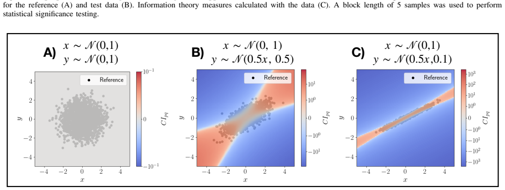
Simulate reference data with a linear dependence $y = 0.5x + \text{noise}$ and test data with a sinusoidal dependence over a similar x-range: the paper's Fig. 3B predicts a strongly negative cross MI, showing that any X-Y dependence not present in the reference is read as surprise rather than dependence. A second check: push test data outside the reference's x-range (as in Fig. 3A) and estimate cross MI with a model-free estimator; the estimate should show high variance (the paper reports standard deviation 0.26), confirming the support assumption.
Extended reading notes
Core claim
The central discovery is that the cross mutual information defined by $\mathrm{CI}_{pq} = \mathbb{E}_{x,y\sim p}[\log(q(x,y)/q(x)q(y))]$ gives the expected strength of dependence between X and Y in test samples drawn from p, as judged by a reference model q. Because only q needs to be well-estimated, the measure works when p is represented by few samples or a single point; the test data enters only through the empirical average of the pointwise (local) MI computed under q. The paper demonstrates in simulation that cross MI can separate the dependence expressed in a conditioned subset of a system from the dependence of the full ensemble, that it can go negative when test data is 'surprising' relative to q, and that a Gaussian model of q makes cross MI a direct generalisation of cross-validated sum-of-squared-residuals while retaining the chain rule.
Load-bearing premise
The load-bearing premise is that a well-sampled reference distribution q is available that fully spans the accessible regions of the system's probability space, so that test data falls inside the reference's support; otherwise cross MI becomes sensitive to the estimator and unreliable.
Editorial extensions
If this is right
- With a fixed reference distribution, cross MI can be tracked online, sample by sample, without waiting to accumulate enough test data to estimate p.
- Comparing cross MI across conditions removes the synergy and redundancy distortions that conditional MI inherits from conditioning on the condition variable.
- A negative cross MI signals that the test data is surprising relative to the reference, either because it lies outside the reference's support or follows a different dependency.
- For Gaussian reference models, cross MI provides a normalised version of cross-validated prediction error that satisfies the chain rule over predictors.
- The construction extends directly to conditional MI, transfer entropy, and active information storage, yielding 'cross' versions of those measures.
Reading between the lines
- One testable extension is change-point detection: with a fixed reference q, a running cross MI over short windows should rise or fall sharply when the system switches condition, and the sign pattern may identify which condition was entered.
- Since cross MI is an expectation of a local score, it can be decomposed per sample; the distribution of those sample-level scores, not just the mean, may distinguish typical from atypical test data more sensitively than the scalar CI.
- If cross MI is computed with a reference built from a long 'in the wild' recording, it could serve as a normalisation for task-based neuroimaging connectomics: each task condition is scored against the ensemble rather than analysed in isolation, and comparisons across subjects would require careful matching of reference supports.
- The ratio sensitivity noted in Appendix C suggests a practical caution: when test data is folded into the reference, cross MI changes with the number of test samples, so comparing two systems requires equal-size or weighted references.
Signed reviews
Editorial analysis
A structured set of objections, weighed in public.
Referee Report
Summary. The paper introduces cross mutual information (cross MI), defined in Eq. (4) as CI_pq = E_{(x,y)~p(x,y)}[log(q(x,y)/(q(x)q(y)))], which measures how strongly the X-Y dependence encoded in a reference distribution q is expressed in test data sampled from p. The authors derive basic properties (CI_pp = I_p, zero when q factorizes, possible negativity), present simulation studies with KSG estimation for supported and unsupported reference distributions, give a Gaussian closed form, and relate the measure to linear-regression residuals. They also propose permutation significance tests for MI, differences in MI, and cross MI, with the stated goal of handling non-stationary and online data. The mathematical definition and the Gaussian derivation are straightforward and appear correct.
Significance. If taken as a descriptive statistic, cross MI is a useful, parameter-free way to compare pairwise dependence across conditions without estimating the test distribution, and the paper provides an analytic Gaussian form plus public code. The paper's stronger inferential claim, however, depends on the significance test in Appendix A, and that test is degenerate for the limited-test-data (online) setting that motivates the paper. The core measure may still be valuable, but the statistical procedure needs repair before the online-data claims can be supported.
major comments (1)
- [Appendix A, 'Cross MI: is |CI_pq| non-zero?'] The permutation test proposed for limited test data is degenerate and tests the wrong null. In Eq. (4), CI_pq is an expectation over p of log(q(x,y)/(q(x)q(y))). If the reference x is block-shuffled, the surrogate reference joint is, up to finite-sample estimation error, q(x)q(y), so every surrogate pointwise term is log(q(x)q(y)/(q(x)q(y))) = 0. The null distribution therefore collapses to a point mass at zero (or, with a plug-in estimator, to estimator noise around zero). Any non-zero estimate of CI_pq, including pure estimator noise, will be declared significant, so false positives are not controlled. This invalidates the online-data significance testing advertised in Sec. I and used in Fig. 1C ('not statistically significant (see Appendix A)'). A valid test of 'no dependence in the test data' must permute the test x-y pairing while keeping the reference q fixed; when only one test point is available, no nonparametric null can be formed in this way, and the text should either provide an alternative procedure or explicitly withdraw the inferential claim for single online points.
minor comments (6)
- [Sec. II-B] The word 'Cruicially' should be 'Crucially'.
- [Fig. 2 caption] 'Difference choices for the reference data' should be 'Different choices for the reference data'.
- [Sec. IV-C] The phrase 'the the X-Y dependence' contains a duplicated 'the'.
- [Sec. IV-A] The proposed nearest-neighbour distance check for whether the reference distribution supports the test data is informal; specifying a concrete threshold or validation procedure would make the limitation operational.
- [Sec. III and Fig. 1] The notation alternates between CI_pq and Cpq; using a single symbol consistently throughout would improve readability.
- [Appendix A, 'Differences in MI'] The sign-flip procedure randomly assigns system labels with probabilities proportional to block counts; this is not the usual exchangeability permutation and should be justified or replaced by a standard permutation of pooled blocks.
Circularity Check
No significant circularity: cross MI is defined from first principles and the Gaussian/regression forms follow by substitution; the Appendix A online-test issue is a statistical validity problem, not a circular reduction.
full rationale
The central definition, Eq. (4), CI_pq = E_{x,y~p(x,y)}[log(q(x,y)/(q(x)q(y)))], is an expectation of a pointwise quantity over a test distribution against a reference distribution; it is not defined in terms of any quantity it is used to predict. The Gaussian result, Eq. (10), is obtained by substituting q(y|x) ~ N(mu_Y|X, sigma^2_Y|X) and q(y) ~ N(mu_Y, sigma^2_Y) into Eq. (7) and taking the expectation over p; no test-data parameter is fitted and then relabelled as a prediction. The regression discussion in Appendix B derives the sum-of-squared-residuals term from Eq. (10) rather than imposing it. The stated property that I_q=0 implies CI_pq=0 is a consequence of the definition, not an input-output inversion, and the reference-support limitation is explicitly acknowledged in Sec. IV-A and Fig. 3A. Self-citations are peripheral: [12] motivates block-shuffle permutations, [16] is the software used, and [6] and [17] provide background on PID and local MI; none is needed to make Eqs. (4)-(10) true. The one serious concern in the manuscript is not circularity: in Appendix A, for limited test data the authors propose to 'break the dependence in the reference data instead', but by Eq. (4) shuffling the reference x forces every surrogate CI to log(q(x)q(y)/(q(x)q(y)))=0, making the null distribution degenerate. This undermines the online-data significance test, but it is a statistical validity defect in an application of the measure, not a case of the measure's derivation reducing to its own inputs.
Assumptions & free parameters
assumptions (3)
- domain assumption The KSG estimator provides reliable estimates of pointwise MI for the reference distribution at test sample locations.
- domain assumption The reference distribution q is stationary and sufficiently sampled to represent the full probability space of the system.
- domain assumption The conditioning on a condition variable Θ and the decomposition into synergy/redundancy follow the partial information decomposition framework.
Cite this review
Pith. "Pith review of Cross Mutual Information." pith.science (2026). https://pith.science/paper/KF557GCP
@misc{pith2026250715372,
  author       = {Pith},
  title        = {Pith review of: Cross Mutual Information},
  year         = {2026},
  howpublished = {\url{https://pith.science/paper/KF557GCP}},
  note         = {Machine review of arXiv:2507.15372}
}
abstract
Mutual information (MI) is a useful information-theoretic measure to quantify the statistical dependence between two random variables: $X$ and $Y$. Often, we are interested in understanding how the dependence between $X$ and $Y$ in one set of samples compares to another. Although the dependence between $X$ and $Y$ in each set of samples can be measured separately using MI, these estimates cannot be compared directly if they are based on samples from a non-stationary distribution. Here, we propose an alternative measure for characterising how the dependence between $X$ and $Y$ as defined by one set of samples is expressed in another, \textit{cross mutual information}. We present a comprehensive set of simulation studies sampling data with $X$-$Y$ dependencies to explore this measure. Finally, we discuss how this relates to measures of model fit in linear regression, and some future applications in neuroimaging data analysis.
Figures


Figures from the paper (3 more)


Reference graph
Works this paper leans on
- [1]
-
[2]
Esti- mating mutual information
Kraskov, Alexander, Harald St ¨ogbauer, and Peter Grassberger. “Esti- mating mutual information.” Physical Review E-Statistical, Nonlinear, and Soft Matter Physics 69.6 (2004): 066138
work page 2004
-
[3]
Fano, Robert M., and David Hawkins. ”Transmission of information: A statistical theory of communications.” American Journal of Physics 29.11 (1961): 793-794
work page 1961
-
[4]
Probabilistic machine learning: an introduction
Murphy, Kevin P. Probabilistic machine learning: an introduction. MIT press, 2022
work page 2022
-
[5]
Williams, Paul L., and Randall D. Beer. ”Nonnegative decomposition of multivariate information.” arXiv preprint arXiv:1004.2515 (2010)
arXiv 2010
-
[6]
Lizier, Joseph T., et al. ”Information decomposition of target effects from multi-source interactions: Perspectives on previous, current and future work.” Entropy 20.4 (2018): 307
work page 2018
-
[7]
Jeong, Jaeseung, John C. Gore, and Bradley S. Peterson. ”Mutual information analysis of the EEG in patients with Alzheimer’s disease.” Clinical neurophysiology 112.5 (2001): 827-835
work page 2001
-
[8]
Peralta, Joaquin, and Christian Flores. ”Cross Mutual Information Analysis of EEG Signals for Cognitive Task Discrimination.” Brazilian Technology Symposium. Cham: Springer International Publishing, 2021
work page 2021
Show all 35 references
-
[9]
”It’s easier to translate out of english than into it: Measuring neural translation difficulty by cross-mutual information.” arXiv preprint arXiv:2005.02354 (2020)
Bugliarello, Emanuele, et al. ”It’s easier to translate out of english than into it: Measuring neural translation difficulty by cross-mutual information.” arXiv preprint arXiv:2005.02354 (2020)
2020 arXiv
-
[10]
Nasrabadi
Bishop, Christopher M., and Nasser M. Nasrabadi. Pattern recognition and machine learning. V ol. 4. No. 4. New York: springer, 2006
2006
-
[11]
Resampling methods for dependent data
Lahiri, Soumendra Nath. Resampling methods for dependent data. Springer Science & Business Media, 2013
2013
-
[12]
”Assessing the significance of directed and multivariate measures of linear dependence between time series.” Physical Review Research 3.1 (2021): 013145
Cliff, Oliver M., et al. ”Assessing the significance of directed and multivariate measures of linear dependence between time series.” Physical Review Research 3.1 (2021): 013145
2021
-
[13]
Lizier, Joseph T., Mikhail Prokopenko, and Albert Y . Zomaya. ”Local measures of information storage in complex distributed computation.” Information Sciences 208 (2012): 39-54
2012
-
[14]
”Measuring information transfer.” Physical review letters 85.2 (2000): 461
Schreiber, Thomas. ”Measuring information transfer.” Physical review letters 85.2 (2000): 461
2000
-
[15]
Transfer entropy
Bossomaier, Terry, et al. Transfer entropy. Springer International Publishing, 2016
2016
-
[16]
JIDT: An information-theoretic toolkit for studying the dynamics of complex systems
Lizier, Joseph T. “JIDT: An information-theoretic toolkit for studying the dynamics of complex systems.” Frontiers in Robotics and AI 1 (2014): 11
2014
-
[17]
Finn, Conor, and Joseph T. Lizier. ”Probability mass exclusions and the directed components of mutual information.” Entropy 20.11 (2018): 826. APPENDIX A STATISTICAL SIGNIFICANCE TESTING We use statistical significance testing to determine whether the value of the measure we o...
2018
-
[18]
This provides a surrogate x time series
Block shuffle the x time series to break the dependence between X and Y . This provides a surrogate x time series
-
[19]
Calculate MI using the surrogate x time series and the non-permuted y time series
-
[20]
Repeat a number of times to build a null distribution for I = 0
-
[21]
This provides a p-value for |I| > 0
Look up where the MI for the non-permuted data lies in the null distribution. This provides a p-value for |I| > 0. Differences in MI: is ∆Ipq = |Ip − Iq| non-zero?: We are interested in testing whether the observed difference in MI is significantly different from zero. We do t...
-
[22]
6 x[t]=0.8x[t∼1]+π y[t]=0.3y[t∼1]+0.6x[t∼1]+π x[t]=0.8x[t∼1]+π y[t]=0.9x[t∼1]+πA) B) C) Fig
Calculate the local MI for each system condition of interest: iq and ip. 6 x[t]=0.8x[t∼1]+π y[t]=0.3y[t∼1]+0.6x[t∼1]+π x[t]=0.8x[t∼1]+π y[t]=0.9x[t∼1]+πA) B) C) Fig. 4. The proposed statistical significance testing can be applied to autocorrelated data. Simulated data (100 sam...
2000
-
[23]
There may be a different number of blocks for the reference and test system
Separate the local MI into blocks and average the values in each block: ib q and ib p. There may be a different number of blocks for the reference and test system
-
[24]
Randomly assign the system label to each block MI with a probability reflecting the fraction of blocks from each system
-
[25]
Take the difference in the mean across blocks: ∆Ipq = ˜ib p − ˜ib q , where ˜ib q and ˜ib p are the shuffled block MIs and ⟨.⟩ denotes the average
-
[26]
Repeat to build a null distribution for ∆Ipq = 0
-
[27]
This provides a p- value for |∆Ipq| > 0
Look up where the non-permuted difference in MI (∆Ipq) lies in the null distribution. This provides a p- value for |∆Ipq| > 0. Cross MI: is |CI pq| non-zero?: We are interested in whether an observed value for the cross MI is significantly different from zero, indicating there...
-
[28]
Split the x time series in the test (or reference) data into blocks and shuffle to obtain a surrogate x test time series
-
[29]
Note, we also rely on the dependence between X and Y in the reference data being non-zero to obtain a non-zero cross MI - see Sec
Calculate the surrogate cross MI using the surrogate x test time series and non-permuted test y time series along with the non-permuted reference data. Note, we also rely on the dependence between X and Y in the reference data being non-zero to obtain a non-zero cross MI - see Sec. II
-
[30]
Repeat to build a null distribution
-
[31]
fraction of variance unexplained
Look up what percentile the non-permuted cross MI 7 x∼𝒩(0,1) y∼𝒩(0,1) x∼𝒩(1.5,0.4) y∼𝒩(0.5x,0.1) x∼𝒩(0,1) y∼𝒩(0.5x,0.1) x∼𝒩(1.5,0.4) y∼𝒩(0.5x,0.1) x∼𝒩(1,0.5) y∼𝒩(2sin(2πx+ϕ)+1,0.05) x∼𝒩(1,0.5) y∼𝒩(2sin(2πx+ϕ)+1,0.05) A) B) C) D) Fig. 6. The cross MI scales with number of sampl...
2000
-
[32]
the pointwise MI in Eq. (7) is derived as the unique form to measure the information a sample x provides about y given the reference distributions q(y) and q(y|x) fulfilling certain axioms (including a chain rule) [3], and
-
[33]
that such information is a measure of the quality of prediction in terms of how the sample x constrains our expectation of the probabilities for y given x (see e.g. [17]), then one would conclude that the cross MI (in averaging the pointwise MI over the test data) would be the...
-
[34]
Quantitatively, for fixed y (constant q(y)), moving towards the trendline means q(y|x) increases which directly increases iq(x, y) in Eq
The MI increases as we approach the trendline y = βx + γ for the posterior model, since X becomes more strongly predictive of Y using the model along this gradient. Quantitatively, for fixed y (constant q(y)), moving towards the trendline means q(y|x) increases which directly ...
-
[35]
Quantitatively, q(y|x) is fixed along these parallels to the trendline, whilst q(y) decreases along these perpediculars; this directly increases iq(x, y) in Eq
The MI increases along or parallel to the trendline for the posterior model, when moving away from the perpendicular bisector through the variables’ means. Quantitatively, q(y|x) is fixed along these parallels to the trendline, whilst q(y) decreases along these perpediculars; ...
Reviewed August 6, 2026 · model on record in the stance chip above.
Discussion (0). Continue with ORCID to comment.