REVIEW 3 major objections 4 minor 70 references
Impact of Bottleneck Layers and Skip Connections on the Generalization of Linear Denoising Autoencoders
T0 review · 3 major / 4 minor · reviewed 2026-08-07 · deepseek-v4-flash
Pith's one-line read Bottleneck width creates a bias-variance trade-off in linear denoising autoencoders, and skip connections damp the overparameterization peak, according to closed-form test-risk formulas.
desk verdict A real step forward for linear DAE theory, but the skip-connection risk formula in Theorem 3.5 has a spurious 1/c that must be fixed. read the letter →
The pith
A machine-rendered reading of the paper's core claim, the machinery that carries it, and where it could break.
The reading
What carries the argument
The load-bearing object is the closed-form characterization of all critical points of the product-regularized two-layer linear loss: every critical point has the form $\hat W_c = U_{G,I}U_{G,I}^\top YZ^\top(\tilde Z\tilde Z^\top)^{-1}$, and in the ridgeless limit $W_c = P_I(Y)Z^\dagger$, with the global minimizer $W_* = P_{[k]}(X)(X+A)^\dagger$. The risk proofs expand $(X+A)^\dagger$ through a pseudo-inverse perturbation formula and then replace expectations of products of the random matrices $D(P^\top P)^{-1}D$, $K_1^{-1}$, $ZD^{-1}$, and $HH^\top$ by products of expectations, relying on element-wise variances of order $O(1/d)$. For the skip-connection comparison, the paper introduces the rank-$1$ additive model $S=XX^\top+AA^\top$ and proves the alignment ratio identity $E[\langle u_i^A,u_j^S\rangle^2 / \langle u_1,u_j^S\rangle^2] = \Theta\left(\frac{1}{d(\lambda_i^A-\lambda_j^S)^2}\right)$, which is what makes the noise-alignment contribution to the variance parametrically smaller.
What would settle it
Fix a deterministic rank-$r$ signal with well-conditioned spectrum, draw Gaussian training and test noise with variances $\eta_{\mathrm{trn}}^2/d$ and $\eta_{\mathrm{tst}}^2/d$, and train both models to their ridgeless global minimizers. Compare the measured test risk with Eqs. (9) and (10) as $d$ grows with $c$ fixed near $1$: the formulas are falsified if the rescaled variance term $d(c-1)R$ does not converge to $\eta_{\mathrm{tst}}^2 \sum_{j\in[k]} \alpha_j^2/(1+\alpha_j^2)$, or if the skip-connected variance is not smaller by an extra factor of $1/d$.
Extended reading notes
Core claim
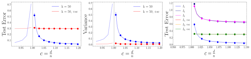
Under a deterministic low-rank signal model with Gaussian noise of variances $\eta_{\mathrm{trn}}^2/d$ and $\eta_{\mathrm{tst}}^2/d$, and with $d \geq n+r$, the paper claims exact control of the test risk of every critical point of the two-layer linear DAE. For the global minimizer $W_* = P_{[k]}(X)(X+A)^\dagger$ without a skip connection, the test risk is $R(W_*, X_{\mathrm{tst}}) = \frac{1}{N_{\mathrm{tst}}}\mathrm{Tr}(JLL^\top) + \frac{\eta_{\mathrm{tst}}^2 c}{d(c-1)}\sum_{j=1}^k \frac{\alpha_j^2}{1+\alpha_j^2} + o(1/d)$, where the diagonal entries of $J$ are $(1+\alpha_i^2)^{-2}$ for the selected directions and $1$ otherwise. The first term falls as $k$ grows, while the second rises, giving the bottleneck width a genuine bias-variance trade-off. With a skip connection, whose training objective is equivalent to predicting the noise $-A$ rather than the clean signal, the paper derives the corresponding risk formula whose variance term is smaller by an extra factor of $1/d$, so the $(c-1)^{-1}$ peak is damped, most visibly in the mildly overparameterized regime. The mechanism is identified in a rank-$1$ additive model $S = XX^\top + AA^\top$: the alignment between singular vectors of the noise and of $S$ is $\Theta(1/d)$ weaker than the alignment between singular vectors of the signal and of $S$, which suppresses the dominant small-eigenvalue contribution to the variance.
Load-bearing premise
The risk formulas rest on the assumption that the random matrices appearing inside the trace concentrate quickly enough that the expectation of a product equals the product of expectations up to $o(1)$ noise; if that joint concentration fails, the closed-form curves could acquire extra terms.
Editorial extensions
If this is right
- For fixed input dimension $d$ and sample size $n$, the test risk as a function of bottleneck width $k$ is U-shaped: larger $k$ lowers bias but raises variance, and the optimal $k$ depends on the overparameterization ratio $c=d/n$.
- Double descent in $d/n$ persists even when the bottleneck is small: the variance term diverges like $(c-1)^{-1}$ as $c$ approaches $1$, so the peak is a genuine feature of the architecture, not of unlimited rank.
- Adding a skip connection changes the effective target from the clean signal to the noise, and the resulting variance term carries an extra $1/d$ factor; this dampens the peak near $c\approx 1$ without eliminating it.
- In the skip-connected model, different critical points have nearly the same test error as the global minimizer, whereas in the bottleneck-only model different critical points can differ substantially in both bias and variance.
- The variance reduction is traced to singular-vector alignment: noise singular vectors align with corrupted-data eigenvectors a factor $\Theta(1/d)$ more weakly than signal singular vectors do, and this suppresses the contribution of the smallest eigenvalues that dominate the variance.
Reading between the lines
- Editorial inference, beyond the paper: the same concentration-plus-pseudo-inverse pipeline should apply to other minimum-norm interpolating autoencoders, such as masked autoencoders where the mask plays the role of the additive noise; the paper does not discuss this extension.
- Editorial inference, beyond the paper: the paper's own remark about a four-layer linear model with the skip connection between hidden layers suggests a direct test of whether the constant $\eta_{\mathrm{tst}}^2$ bias can be removed while preserving the variance damping, since the two-layer input-output skip forces the network to predict full-rank noise.
- Editorial inference, beyond the paper: the theory predicts that the optimal bottleneck width for fixed $n$ should grow with $d$ in the mildly overparameterized regime; a grid search over $k$ and $d$ on low-rank data would provide a sharp quantitative check of the predicted U-shape.
- Editorial inference, beyond the paper: the alignment mechanism likely transfers to nonlinear denoisers trained with denoising score matching, where the effective target is also noise; the paper's linear analysis gives a concrete baseline for how much variance reduction one can attribute to the skip connection alone.
Editorial analysis
A structured set of objections, weighed in public.
Referee Report
Summary. This paper studies two-layer linear denoising autoencoders trained by gradient flow on the squared reconstruction loss with product regularization, in the overparameterized regime d ≥ n + r. For a low-rank Gaussian noise data model (Assumption 3.1), it derives closed-form expressions for all critical points (Theorem 2.1) and specializes them to DAEs with and without an identity skip connection (Corollaries 2.4 and 2.5). It then states asymptotic test-risk formulas (Theorems 3.2 and 3.5) and decomposes them into bias and variance terms, arguing that the bottleneck width k induces a bias-variance trade-off and that skip connections damp the variance peak near c = d/n ≈ 1. Section 4 uses random matrix theory on a rank-1 additive model to explain the variance suppression via weaker eigenvector alignment, and CIFAR-10 experiments support the qualitative curves.
Significance. The paper makes a useful step beyond single-layer analyses: it gives a complete critical-point characterization for two-layer linear DAEs with bottleneck and skip connection, identifies the minimum-norm global minimizer, and produces interpretable closed-form risk formulas. The bias-variance decomposition of Eq. (9) and the variance-damping comparison between Eq. (9) and Eq. (10) are conceptually valuable, and the numerical experiments appear to match the intended predictions. However, the main theorem for the skip-connection model, Theorem 3.5, contains an algebraic error: the stated J_sc is inconsistent with the paper's own Lemma E.13 and with the mean computations in its proof. Because Eq. (10) is advertised in the abstract as one of the two central risk formulas, the paper cannot be accepted without correcting this formula and re-checking the figures that plot it.
major comments (3)
- [Theorem 3.5, Eq. (10), and Lemma E.13] The stated coefficient J_sc does not follow from the paper's own derivation. Lemma E.13 states E∥W_sc X_tst∥²_F = |I_a|/d Tr(((c−1)D²+I_d)(I_r+η_{trn}^{-2}D²)^{-2}LL^T)+O(d^{-1}); substituting this into the decomposition in Eq. (31) yields the bias term |I_a|/(dN_tst) Tr(J_correct LL^T) with J_correct,ii = ((c−1)σ_i²+1)/(1+η_{trn}^{-2}σ_i²)^2. Theorem 3.5 instead has J_sc,ii = (c+(c−1)σ_i²)/(c(1+η_{trn}^{-2}σ_i²)^2), which differs by a factor 1/c on the σ_i² term. The proof of Lemma E.13 also ends with a third, different form ((c−1)D²+cI_d)(cI_r+cη^{-2}D²)^{-2}. The theorem as stated is therefore not established by the preceding argument; please correct Eq. (10), align the closing display of Lemma E.13 with its statement, and verify that the theoretical curves in Figure 3 use the corrected formula.
- [Appendix E.1, Eqs. (28)-(30) and Lemmas E.2-E.13] The central derivations rely on replacing expectations of products of random matrix factors by products of expectations, justified by element-wise variance O(d^{-1}) for each factor. For products of four dependent factors such as D(P^T P)^{-1}D, K_1^{-1}, ZD^{-1}, and HH^T, the error involves joint fourth-order cumulants, not just pairwise variances. The manuscript cites [27] and [11] but does not state or prove a uniform lemma controlling these cross-terms. Since the closed-form risk formulas depend on this concentration step, please provide the missing concentration lemma or an explicit reference with the exact statement used.
- [Section 4, Definition 4.1 and Theorem 4.3] The alignment-suppression theorem is proved for the additive model S=XX^T+AA^T, whereas the DAE actually corresponds to the information-plus-noise model (X+A)(X+A)^T. Remark 4.2 only matches first moments of the two models; it does not imply that eigenvector alignment properties transfer. The paper acknowledges the simplification, but as written the 'origin' of the variance discrepancy is a heuristic supported by a related model, not a theorem for the actual model. Please either prove the analogous statement for (X+A)(X+A)^T (or a precise asymptotic equivalence) or explicitly label this part as a heuristic.
minor comments (4)
- [Appendix E.2, Definition E.14] Defining bias as the component that decreases with k and variance as the component that increases with k makes the bias-variance trade-off true by definition. The concrete decompositions in Eq. (28), Eq. (31), Lemmas E.3/E.4, and E.11/E.12 are the substantive statements; please present Definition E.14 as an interpretive summary rather than a formal definition.
- [Remark F.4] The case j=1 is dismissed 'for brevity' in a proof of a theorem about alignment; since the largest eigenvalue can dominate variance, this case should be either proved or explicitly excluded from the theorem statement.
- [Appendix E, notation] In Appendix E, D is used both as a d×d matrix and as an r×r block, and Lemma E.13 mixes I_d and I_r; please make the dimensions of all identity matrices and diagonal blocks explicit.
- [Theorems 3.2 and 3.5] The theorems state asymptotic o(1/d) and O(1/(dN_tst)) remainders while the text calls the setting 'non-asymptotic'; please clarify whether these are statements about sequences with d,n→∞ or finite-d bounds with explicit constants.
Circularity Check
No significant circularity: the risk formulas are derived from explicit critical-point expressions and concentration lemmas, not from fitted parameters or self-citations.
full rationale
The paper's derivation chain is self-contained in the sense relevant to circularity analysis. The closed-form risk formulas in Theorems 3.2 and 3.5 are obtained by substituting the explicitly characterized critical points W_c = P_Ix(X)(X+A)^+ and W^sc_c = -P_Ia(A)(X+A)^+ into the test-risk definitions, expanding the pseudo-inverse via the Woodbury-type identity from [45], and then applying concentration arguments (largely inherited from [27] and [38]) to replace expectations of products of random matrices by products of expectations. No parameter is fitted to data, no 'prediction' is defined in terms of a fitted value, and the formulas are not assumed as ansatze. The prior results [27, 38] are by different authors, so there is no load-bearing self-citation chain. The only passage that could raise a definitional concern is Definition E.14, which defines bias as the component that decreases with bottleneck width k and variance as the component that increases with k; this is tautological as a labeling device, but it is applied after the monotonicity of the terms in Eq. (9) and Eq. (10) is already established, and it does not enter the derivation of the risk formulas. The skeptic's suspected 1/c inconsistency in Lemma E.13/Theorem 3.5 is a mathematical correctness or proof-consistency issue, not a circularity: Eq. (10) is not equivalent to its inputs by construction, and correcting an algebraic factor would not change the derivation structure. Accordingly, the paper earns a 0 circularity score.
Assumptions & free parameters
assumptions (6)
- domain assumption The clean data X is a deterministic low-rank matrix with rank r ≪ d,n, spectral norm Θ(1), and well-conditioned nonzero singular values; test data lies in the same subspace.
- domain assumption The additive noise matrices A and A_tst have i.i.d. Gaussian entries with variance η²_trn/d and η²_tst/d.
- domain assumption X+A has full column rank n (holds almost surely when d ≥ n).
- domain assumption The nonzero eigenvalues of XX^T and AA^T have multiplicity one.
- domain assumption Gradient flow converges to the global minimizer of the regularized loss; the λ→0 ridgeless limit selects the minimum-norm solution.
- standard math Standard random matrix theory results hold, including the Marchenko-Pastur law, concentration of quadratic forms, and resolvent identities.
Cite this review
Pith. "Pith review of Impact of Bottleneck Layers and Skip Connections on the Generalization of Linear Denoising Autoencoders." pith.science (2026). https://pith.science/paper/KF6JB2ZF
@misc{pith2026250524668,
  author       = {Pith},
  title        = {Pith review of: Impact of Bottleneck Layers and Skip Connections on the Generalization of Linear Denoising Autoencoders},
  year         = {2026},
  howpublished = {\url{https://pith.science/paper/KF6JB2ZF}},
  note         = {Machine review of arXiv:2505.24668}
}
read the original abstract
Modern deep neural networks exhibit strong generalization even in highly overparameterized regimes. Significant progress has been made to understand this phenomenon in the context of supervised learning, but for unsupervised tasks such as denoising, several open questions remain. While some recent works have successfully characterized the test error of the linear denoising problem, they are limited to linear models (one-layer network). In this work, we focus on two-layer linear denoising autoencoders trained under gradient flow, incorporating two key ingredients of modern deep learning architectures: A low-dimensional bottleneck layer that effectively enforces a rank constraint on the learned solution, as well as the possibility of a skip connection that bypasses the bottleneck. We derive closed-form expressions for all critical points of this model under product regularization, and in particular describe its global minimizer under the minimum-norm principle. From there, we derive the test risk formula in the overparameterized regime, both for models with and without skip connections. Our analysis reveals two interesting phenomena: Firstly, the bottleneck layer introduces an additional complexity measure akin to the classical bias-variance trade-off -- increasing the bottleneck width reduces bias but introduces variance, and vice versa. Secondly, skip connection can mitigate the variance in denoising autoencoders -- especially when the model is mildly overparameterized. We further analyze the impact of skip connections in denoising autoencoder using random matrix theory and support our claims with numerical evidence.
Figures

Reference graph
Works this paper leans on
-
[27]
Double Descent and Overfitting under Noisy Inputs and Distribution Shift for Linear Denoisers
Chinmaya Kausik, Kashvi Srivastava, and Rishi Sonthalia. Double Descent and Overfitting under Noisy Inputs and Distribution Shift for Linear Denoisers. 2024. arXiv: 2305.17297 [cs.LG]. URL: https://arxiv.org/abs/2305.17297
arXiv 2024
-
[11]
On the Exact Covariance of Products of Random Variables
George W. Bohrnstedt and Arthur S. Goldberger. “On the Exact Covariance of Products of Random Variables”. In: Journal of the American Statistical Association 64.328 (1969), pp. 1439–1442. ISSN : 01621459, 1537274X. URL: http : / / www . jstor . org / stable / 2286081 (visited on 08/10/2024)
work page 1969
-
[1]
The loss landscape of deep linear neural networks: a second-order analysis
El Mehdi Achour, François Malgouyres, and Sébastien Gerchinovitz. The loss landscape of deep linear neural networks: a second-order analysis. 2024. arXiv: 2107.13289 [math.ST]. URL: https://arxiv.org/abs/2107.13289
work page Pith review arXiv 2024
-
[2]
A Random Matrix Perspective on Mixtures of Nonlinearities in High Dimensions
Ben Adlam, Jake A. Levinson, and Jeffrey Pennington. “A Random Matrix Perspective on Mixtures of Nonlinearities in High Dimensions”. In: Proceedings of The 25th International Conference on Artificial Intelligence and Statistics. Ed. by Gustau Camps-Valls, Francisco J. R. Ruiz, and Isabel Valera. V ol. 151. Proceedings of Machine Learning Research. PMLR, 2...
work page 2022
-
[3]
Lars Valerian Ahlfors and Lars V Ahlfors. Complex analysis. V ol. 3. McGraw-Hill New York, 1979
work page 1979
-
[4]
Generalization of two-layer neural networks: An asymptotic viewpoint
Jimmy Ba et al. “Generalization of two-layer neural networks: An asymptotic viewpoint”. In: International conference on learning representations. 2020
work page 2020
-
[5]
High-dimensional analysis of double descent for linear regression with random projections
Francis Bach. High-dimensional analysis of double descent for linear regression with random projections. 2023. arXiv: 2303.01372 [cs.LG] . URL: https://arxiv.org/abs/2303. 01372
work page Pith review arXiv 2023
-
[6]
Spectral analysis of large dimensional random matrices
Zhidong Bai and Jack W Silverstein. Spectral analysis of large dimensional random matrices. V ol. 20. Springer, 2010
work page 2010
Show all 70 references
-
[7]
Silverstein
Jinho Baik and Jack W. Silverstein. Eigenvalues of Large Sample Covariance Matrices of Spiked Population Models. 2004. arXiv: math/0408165 [math.ST]. URL: https://arxiv. org/abs/math/0408165
2004 arXiv
-
[8]
Neural networks and principal component analysis: Learning from examples without local minima
Pierre Baldi and Kurt Hornik. “Neural networks and principal component analysis: Learning from examples without local minima”. In: Neural networks 2.1 (1989), pp. 53–58
1989
-
[9]
Benign overfitting in linear regression
Peter L. Bartlett et al. “Benign overfitting in linear regression”. In:Proceedings of the National Academy of Sciences 117.48 (Apr. 2020), pp. 30063–30070. ISSN : 1091-6490. DOI: 10.1073/ pnas.1907378117. URL: http://dx.doi.org/10.1073/pnas.1907378117
2020 doi
-
[10]
Reconciling modern machine-learning practice and the classical bias–variance trade-off
Mikhail Belkin et al. “Reconciling modern machine-learning practice and the classical bias–variance trade-off”. In: Proceedings of the National Academy of Sciences 116.32 (2019). ISSN : 1091-6490. DOI: 10.1073/pnas.1903070116 . URL: http://dx.doi.org/10. 1073/pnas.1903070116
2019 doi
-
[12]
Random Matrix Methods for Machine Learning
Romain Couillet and Zhenyu Liao. Random Matrix Methods for Machine Learning. https: //zhenyu-liao.github.io/book/ . Cambridge University Press, 2022. DOI: 10.1017/ 9781009128490
2022
-
[13]
High-dimensional asymptotics of denoising autoencoders
Hugo Cui and Lenka Zdeborová. “High-dimensional asymptotics of denoising autoencoders”. In: Advances in Neural Information Processing Systems 36 (2023), pp. 11850–11890
2023
-
[14]
A U-turn on Double Descent: Rethinking Parameter Counting in Statistical Learning
Alicia Curth, Alan Jeffares, and Mihaela van der Schaar. “A U-turn on Double Descent: Rethinking Parameter Counting in Statistical Learning”. In: Thirty-seventh Conference on Neural Information Processing Systems. 2023. URL: https://openreview.net/forum? id=O0Lz8XZT2b
2023
-
[15]
Procedures for Reduced-Rank Regression
P. T. Davies and M. K-S. Tso. “Procedures for Reduced-Rank Regression”. In: Journal of the Royal Statistical Society. Series C (Applied Statistics) 31.3 (1982), pp. 244–255. ISSN : 00359254, 14679876. URL: http : / / www . jstor . org / stable / 2347998(visited on 01/30/2025)
1982
-
[16]
On the empirical distribution of eigenvalues of large dimensional information-plus-noise-type matrices
R Brent Dozier and Jack W Silverstein. “On the empirical distribution of eigenvalues of large dimensional information-plus-noise-type matrices”. In: Journal of Multivariate Analysis 98.4 (2007), pp. 678–694
2007
-
[17]
Probability: theory and examples
Rick Durrett. Probability: theory and examples. V ol. 49. Cambridge university press, 2019. 10
2019
-
[18]
The approximation of one matrix by another of lower rank
Carl Eckart and Gale Young. “The approximation of one matrix by another of lower rank”. In: Psychometrika 1.3 (1936), pp. 211–218
1936
-
[19]
The rank of a random matrix
Xinlong Feng and Zhinan Zhang. “The rank of a random matrix”. In: Applied mathematics and computation 185.1 (2007), pp. 689–694
2007
-
[20]
No Double Descent in Prin- cipal Component Regression: A High-Dimensional Analysis
Daniel Gedon, Antonio H. Ribeiro, and Thomas B. Schön. “No Double Descent in Prin- cipal Component Regression: A High-Dimensional Analysis”. In: Proceedings of the 41st International Conference on Machine Learning. Ed. by Ruslan Salakhutdinov et al. V ol. 235. Proceedings of M...
2024
-
[21]
Asymptotic errors for convex penalized linear regression beyond Gaussian matrices
Cédric Gerbelot, Alia Abbara, and Florent Krzakala. Asymptotic errors for convex penalized linear regression beyond Gaussian matrices. 2020. arXiv: 2002.04372 [stat.ML] . URL: https://arxiv.org/abs/2002.04372
2020 arXiv
-
[22]
Surprises in High-Dimensional Ridgeless Least Squares Interpolation
Trevor Hastie et al. Surprises in High-Dimensional Ridgeless Least Squares Interpolation
-
[23]
Deep Residual Learning for Image Recognition
Kaiming He et al. Deep Residual Learning for Image Recognition. 2015. arXiv: 1512.03385 [cs.CV]. URL: https://arxiv.org/abs/1512.03385
2015 arXiv
-
[24]
Denoising Diffusion Probabilistic Models
Jonathan Ho, Ajay Jain, and Pieter Abbeel. Denoising Diffusion Probabilistic Models. 2020. arXiv: 2006.11239 [cs.LG]. URL: https://arxiv.org/abs/2006.11239
2020 arXiv
-
[25]
No Double Descent in Self-Supervised Learning
Dulhan Hansaja Jayalath, Alisia Maria Lupidi, and Yonatan Gideoni. No Double Descent in Self-Supervised Learning . 2023. URL: https : / / openreview . net / forum ? id = qNJRvdKDGYg
2023
-
[26]
On the Distribution of the Largest Eigenvalue in Principal Components Analysis
Iain M. Johnstone. “On the Distribution of the Largest Eigenvalue in Principal Components Analysis”. In: The Annals of Statistics 29.2 (2001), pp. 295–327. ISSN : 00905364, 21688966. URL: http://www.jstor.org/stable/2674106 (visited on 01/26/2025)
2001
-
[28]
Deep Learning without Poor Local Minima
Kenji Kawaguchi. Deep Learning without Poor Local Minima . 2016. arXiv: 1605.07110 [stat.ML]. URL: https://arxiv.org/abs/1605.07110
2016 arXiv
-
[29]
Learning multiple layers of features from tiny images
Alex Krizhevsky, Geoffrey Hinton, et al. “Learning multiple layers of features from tiny images”. In: (2009)
2009
-
[30]
Does Double Descent Occur in Self- Supervised Learning?
Alisia Lupidi, Yonatan Gideoni, and Dulhan Jayalath. “Does Double Descent Occur in Self- Supervised Learning?” In: arXiv preprint arXiv:2307.07872 (2023)
2023 arXiv
-
[31]
Reduced rank ridge regression and its kernel extensions
Ashin Mukherjee and Ji Zhu. “Reduced rank ridge regression and its kernel extensions”. In: Statistical analysis and data mining: the ASA data science journal 4.6 (2011), pp. 612–622
2011
-
[32]
Deep Double Descent: Where Bigger Models and More Data Hurt
Preetum Nakkiran et al. Deep Double Descent: Where Bigger Models and More Data Hurt
-
[33]
Learning dynamics of linear denoising autoencoders
Arnu Pretorius, Steve Kroon, and Herman Kamper. “Learning dynamics of linear denoising autoencoders”. In: International Conference on Machine Learning. PMLR. 2018, pp. 4141– 4150
2018
-
[34]
Multiple Descents in Unsupervised Learning: The Role of Noise, Domain Shift and Anomalies
Kobi Rahimi, Tom Tirer, and Ofir Lindenbaum. “Multiple Descents in Unsupervised Learning: The Role of Noise, Domain Shift and Anomalies”. In:arXiv preprint arXiv:2406.11703 (2024)
2024
-
[35]
U-Net: Convolutional Networks for Biomedical Image Segmentation
Olaf Ronneberger, Philipp Fischer, and Thomas Brox. U-Net: Convolutional Networks for Biomedical Image Segmentation. 2015. arXiv: 1505.04597 [cs.CV]. URL: https://arxiv. org/abs/1505.04597
2015 arXiv
-
[36]
Smallest singular value of a random rectangular matrix
Mark Rudelson and Roman Vershynin. “Smallest singular value of a random rectangular matrix”. In: Communications on Pure and Applied Mathematics: A Journal Issued by the Courant Institute of Mathematical Sciences 62.12 (2009), pp. 1707–1739
2009
-
[37]
On the Empirical Distribution of Eigenvalues of a Class of Large Dimensional Random Matrices
J.W. Silverstein and Z.D. Bai. “On the Empirical Distribution of Eigenvalues of a Class of Large Dimensional Random Matrices”. In: Journal of Multivariate Analysis 54.2 (1995), pp. 175–192. ISSN : 0047-259X. DOI: https://doi.org/10.1006/jmva.1995.1051. URL: https://www.science...
1995
-
[38]
Training Data Size Induced Double Descent For Denoising Neural Networks and the Role of Training Noise Level
Rishi Sonthalia and Raj Rao Nadakuditi. Training Data Size Induced Double Descent For Denoising Neural Networks and the Role of Training Noise Level . 2022. URL: https:// openreview.net/forum?id=5ALGcXpmFyC
2022
-
[39]
Topics in random matrix theory
Terence Tao. Topics in random matrix theory. V ol. 132. American Mathematical Soc., 2012. 11
2012
-
[40]
Dimensionality Reduction, Regulariza- tion, and Generalization in Overparameterized Regressions
Ningyuan Teresa, David W. Hogg, and Soledad Villar. “Dimensionality Reduction, Regulariza- tion, and Generalization in Overparameterized Regressions”. In:SIAM Journal on Mathematics of Data Science 4.1 (Feb. 2022), pp. 126–152. ISSN : 2577-0187. DOI: 10.1137/20m1387821. URL: h...
2022 doi
-
[41]
Pure and Spurious Critical Points: a Geomet- ric Study of Linear Networks
Matthew Trager, Kathlén Kohn, and Joan Bruna. Pure and Spurious Critical Points: a Geomet- ric Study of Linear Networks. 2020. arXiv: 1910.01671 [cs.LG] . URL: https://arxiv. org/abs/1910.01671
2020 arXiv
-
[42]
Why are Big Data Matrices Approximately Low Rank?
Madeleine Udell and Alex Townsend. Why are Big Data Matrices Approximately Low Rank?
-
[43]
High-dimensional probability: An introduction with applications in data science
Roman Vershynin. High-dimensional probability: An introduction with applications in data science. V ol. 47. Cambridge university press, 2018
2018
-
[44]
Stacked denoising autoencoders: Learning useful representations in a deep network with a local denoising criterion
Pascal Vincent et al. “Stacked denoising autoencoders: Learning useful representations in a deep network with a local denoising criterion.” In: Journal of machine learning research11.12 (2010)
2010
-
[45]
The weighted Moore–Penrose inverse of modified matrices
Yimin Wei. “The weighted Moore–Penrose inverse of modified matrices”. In:Applied Math- ematics and Computation 122.1 (2001), pp. 1–13. ISSN : 0096-3003. DOI: https://doi. org/10.1016/S0096- 3003(00)00007- 2 . URL: https://www.sciencedirect.com/ science/article/pii/S0096300300000072
2001 doi
-
[46]
Optimal exact least squares rank minimization
Shuo Xiang et al. “Optimal exact least squares rank minimization”. In: Proceedings of the 18th ACM SIGKDD international conference on Knowledge discovery and data mining. 2012, pp. 480–488
2012
-
[47]
Critical Points of Neural Networks: Analytical Forms and Landscape Properties
Yi Zhou and Yingbin Liang. Critical Points of Neural Networks: Analytical Forms and Landscape Properties. 2017. arXiv: 1710.11205 [stat.ML]. URL: https://arxiv.org/ abs/1710.11205. Appendix We include additional material in the appendix. Section A discusses further related wor...
2017 arXiv
-
[51]
The above eq
(Empirical Spectral Measure). The above eq. (13) is formally known as Empirical Spectral Measure, and for a symmetric matrix M ∈ Rd×d, it is defined as µM = 1 d dX i=1 δλM i
-
[52]
For a real probability measureµ with support supp(µ), the Stieltjes Transform of µ is defined as mµ(α) = Z 1 x − α dµ(x), α ∈ C\supp(µ)
(Stieltjes Transform). For a real probability measureµ with support supp(µ), the Stieltjes Transform of µ is defined as mµ(α) = Z 1 x − α dµ(x), α ∈ C\supp(µ). 14 Note that the stieltjes transform of the empirical spectral measure is given by, mµM (α) = Z 1 x − α dµM(x) = 1 d ...
-
[53]
Let A ∈ Rp×p, and x, y ∈ Rp
(Sherman-Morrison Formula). Let A ∈ Rp×p, and x, y ∈ Rp. For 1 + yT Ax ̸= 0, we have that (A + xyT )−1 = A−1 − A−1xyT A−1 1+yT Ax
-
[54]
For α ∈ C\R+, let ˜Q(α) = ˜A ˜AT − αId −1 = NP i=1 ˜ai˜aT i − αId −1 , where ˜A ∈ Rd×N is a i.i.d real gaussian random matrix, whose entries are sampled from N (0, 1)
(Concentration of Quadratic Forms, Gaussian case). For α ∈ C\R+, let ˜Q(α) = ˜A ˜AT − αId −1 = NP i=1 ˜ai˜aT i − αId −1 , where ˜A ∈ Rd×N is a i.i.d real gaussian random matrix, whose entries are sampled from N (0, 1). Let ˜Q−j(α) be ˜Q(α) with j-th row and column removed. The...
-
[55]
For symmetric and positive semi-definite B, M ∈ Rd×d, and α ∈ C\R+, let M := hP j=1 lixixT i for fixed h, and li ∈ R, xi ∈ Rd
(Minimal Effect of Finite-Rank Perturbations Inside a Trace, due to [37, Lemma 2.6]). For symmetric and positive semi-definite B, M ∈ Rd×d, and α ∈ C\R+, let M := hP j=1 lixixT i for fixed h, and li ∈ R, xi ∈ Rd. Then, we have that | Tr (B − αI)−1 − (B + M − αI)−1 | ≤ h Im(α) ...
-
[56]
For A ∈ Rp×q, B ∈ Rq×p, and λ ∈ R\{0}
(Weinstein-Aronszajn Identity). For A ∈ Rp×q, B ∈ Rq×p, and λ ∈ R\{0}. Then, we have that det(AB − λIp) = (−λ)p−qdet(BA − λIq)
-
[57]
For A ∈ Rp×p, U ∈ Rp×q, V ∈ Rq×p, we have that (A + UVT )−1 = A−1 − A−1U(Iq + VT A−1U)−1VT A−1
(Woodbury Identity). For A ∈ Rp×p, U ∈ Rp×q, V ∈ Rq×p, we have that (A + UVT )−1 = A−1 − A−1U(Iq + VT A−1U)−1VT A−1. C.2 Getting Subspace Information One useful property of the resolvent and the Stieltjes transform is their connection to the eigenstructure of a random matrix. ...
-
[58]
Furthermore, B has rB eigenvalues equal to 1 and the rest equal to 0
B ∈ R(D−rG)×(D−rG) is defined as B := B1B⊤ 1 , where B1 = ((U⊤ GU ˆW2 )i,j)rG+1≤i≤d,rG+1≤j≤d. Furthermore, B has rB eigenvalues equal to 1 and the rest equal to 0
-
[59]
D ∈RrG×rG is a diagonal matrix with its diagonal elements consist of rD number of 1’s and rG − rD number of 0’s
-
[60]
rD + rB = r ˆW2 . Proof. We analyze the conditions (17) and (18) further. Consider the eigendecomposition of G, given by G = UGΛGU⊤ G, and the singular value decomposition of ˆW2, given by ˆW2 = U ˆW2 Σ ˆW2 V⊤ ˆW2 . Then, PU⊤ G ˆW2 = U⊤ G ˆW2(U⊤ G ˆW2)† = U⊤ G ˆW2 ˆW† 2UG = U⊤...
-
[61]
Let (I, B) a tuple, such that |I| + rB = k, for I ∈ I. Then, for ˆW2 and ˆW1 define critical points for (3) if and only if there exist an invertible matrix C ∈ Rk×k and a tuple (I, B) such that ˆW2 and ˆW1 satisfy that: for |I| < k, ˆW2 = UG,I U2 ˜UB1 C, ˆW1 = C−1 UG,I U2 ˜UB1...
-
[62]
Furthermore, assume rZ = n
For some invertible matrix C ∈ Rrk×rk, global minimizers ˆW∗ 2, ˆW∗ 1 are given by ˆW∗ 2 = UG,kC ˆW∗ 1 = C−1U⊤ G,kYZ⊤( ˜Z ˜Z⊤)−1. Furthermore, assume rZ = n. Then the global minimizer W∗ in the ridgeless case is given uniquely4 by, W∗ = lim λ→0 ˆW∗ 2 ˆW∗ 1 = Pk(Y)Z†
-
[63]
For λ >0, we have an unique global minimizer in terms of ˆW∗ = ˆW∗ 2 ˆW∗
-
[64]
⇐" direction of the proof follows from a straightforward calculation, and we therefore omit the details. For the
On the other hand, at λ = 0, there are multiple global minimizers. But for the both cases, it satisfies that all the critical points other than global minima are saddle points. In other words, all the local minima are global minima and other critical points are saddle points. ...
-
[65]
Due to the fact that AI a A†(AI a A†)⊤ = UATaU⊤ A = AI a A†, we have that − Tr(AI a A†(Wsc c )⊤) = Tr(AI a A†(AI a A†)⊤) − Tr(AI a A†H⊤(K1)−1H)− Tr(AI a A†H⊤K−⊤ 1 Z(P⊤P)−⊤D ˜U⊤)
Distributing −AI a A†: For a notational convenience, we define Ta = 1 if i ∈ I a 0 otherwise. Due to the fact that AI a A†(AI a A†)⊤ = UATaU⊤ A = AI a A†, we have that − Tr(AI a A†(Wsc c )⊤) = Tr(AI a A†(AI a A†)⊤) − Tr(AI a A†H⊤(K1)−1H)− Tr(AI a A†H⊤K−⊤ 1 Z(P⊤P)−⊤D ˜U⊤). Note...
-
[66]
The second term has also mean 0 due to Lemma E.9, thus only the variance needs to be bounded for this term
Distributing −AI a A† ˜UDP†: This is − Tr(AI a A† ˜UDP†(Wsc c )⊤) = Tr(AI a A† ˜UDP†( ˜UDP†)⊤) − Tr(AI a A† ˜UDP†(P†)⊤Z⊤K−⊤ 1 H)− Tr(AI a A† ˜UDP†(P†)⊤Z⊤K−⊤ 1 Z(P⊤P)−⊤D ˜U⊤) Note that some terms do not appear here due to Lemma E.8. The second term has also mean 0 due to Lemma ...
-
[67]
The first term is, from Lemma E.7, and Lemma 8 of [27], − Tr(AI a A†H⊤K−1 1 H) = − |I a| n η2 trn c Tr((η2 trnD−2 + Ir)−1) + o |I a| n
Distributing AI a A†H⊤K−1 1 H: This is Tr(AI a A†H⊤K−1 1 H(Wsc c )⊤) = − Tr(AI a A†H⊤K−1 1 H) + Tr(AI a A†H⊤K−1 1 HH⊤K−1 1 H)+ Tr(AI a A†H⊤K−1 1 HH⊤K−1 1 Z(P⊤P)−1D ˜U⊤) Again, using Lemma E.8, some terms are filtered out. The first term is, from Lemma E.7, and Lemma 8 of [27],...
-
[68]
The first term has zero mean, as shown in Lemma E.9
Distributing AI a A†H⊤K−1 1 ZP†: This is Tr(AI a A†H⊤K−1 1 ZP†(Wsc c )⊤) = − Tr(AI a A†H⊤K−1 1 ZP†(P†)⊤DU⊤)+ Tr(AI a A†H⊤K−1 1 ZP†(P†)⊤Z⊤K−1 1 H)+ Tr(AI a A†H⊤K−1 1 ZP†(P†)⊤Z⊤K−1 1 Z(P⊤P)−1DU⊤) From this point onward, since the proof follows a similar structure to previous arg...
-
[69]
For the element-wise variance, Lemma E.3 and Lemmas 4, 6, 7, and 8 from [27] imply that it is of order o(1)
Distributing AI a A† ˜UD(P⊤P)−1Z⊤K−1 1 H: This is Tr(AI a A† ˜UD(P⊤P)−1Z⊤K−1 1 H(Wsc c )⊤) = − Tr(AI a A† ˜UD(P⊤P)−1Z⊤K−1 1 H)− Tr(AI a A† ˜UD(P⊤P)−1Z⊤K−1 1 HH⊤K−1 1 H)+ Tr(AI a A† ˜UD(P⊤P)−1Z⊤K−1 1 HH⊤K−1 1 Z(P⊤P)−1D ˜U⊤) The first and second terms have zero mean, due to Lemm...
-
[70]
Distributing AI a A†UD(P⊤P)−1Z⊤K−1 1 ZP†: This is Tr(AI a A† ˜UD(P⊤P)−1Z⊤K−1 1 ZP†(Wsc c )⊤) = − Tr(AI a A† ˜UD(P⊤P)−1Z⊤K−1 1 ZP†(P†)⊤D ˜U⊤)+ Tr(AI a A† ˜UD(P⊤P)−1Z⊤K−1 1 ZP†(P†)⊤Z⊤K−1 1 H)+ Tr(AI a A† ˜UD(P⊤P)−1Z⊤K−1 1 ZP†(P†)⊤Z⊤K−1 1 Z(P⊤P)−1D ˜U⊤) The second term has zero m...
-
[2018]
URL: https://arxiv.org/abs/1705.07474
arXiv: 1705.07474 [cs.LG]. URL: https://arxiv.org/abs/1705.07474
-
[2019]
URL: https://arxiv.org/abs/1912.02292
arXiv: 1912.02292 [cs.LG]. URL: https://arxiv.org/abs/1912.02292
1912 arXiv
-
[2020]
URL: https://arxiv.org/abs/1903.08560
arXiv: 1903.08560 [math.ST]. URL: https://arxiv.org/abs/1903.08560
1903 arXiv
Reviewed August 7, 2026 · model on record in the stance chip above.
Discussion (0). Sign in to comment.