REVIEW 3 major objections 6 minor 35 references
Dynamics of observables in a $q$-deformed harmonic oscillator
T0 review · 3 major / 6 minor · reviewed 2026-08-14 · deepseek-v4-flash
Pith's one-line read The q-deformed harmonic oscillator can be periodic, quasi-periodic, or chaotic depending on q and the coherent amplitude.
desk verdict The q-deformed oscillator has a pure point spectrum and bounded X, P, so the reported positive Lyapunov exponents are numerical artifacts; Eq. (10) also has a phase-factor error. The paper is readable but the central claim doesn't survive. read the letter →
The pith
A machine-rendered reading of the paper's core claim, the machinery that carries it, and where it could break.
The reading
What carries the argument
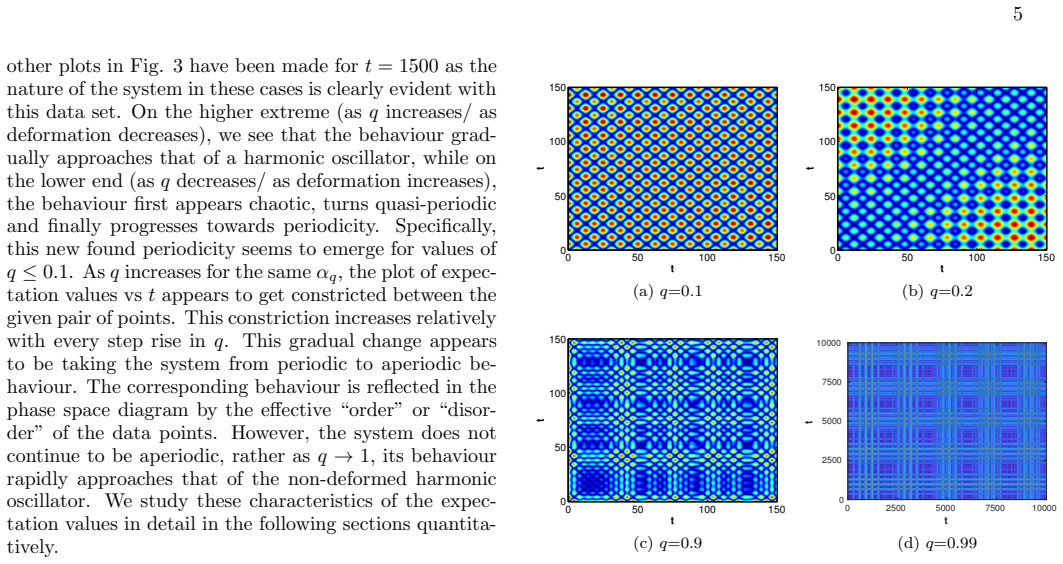
The engine of the paper is the q-number $[n] = (1 - q^{2n})/(1 - q^2)$, which replaces $n$ in the ladder-operator relations $A|n\rangle_q = \sqrt{[n]}\,|n-1\rangle_q$ and $A^\dagger|n\rangle_q = \sqrt{[n+1]}\,|n+1\rangle_q$. This q-number makes the energy spectrum non-linear and produces multi-frequency time dependence in the coherent-state expectation values. The other load-bearing piece is the time-evolved deformed coherent state in Eq. (10), whose phase factors $e^{-it/2} e^{-it[n](1+q^2)/2}$ generate the sums in Eqs. (12)-(13) for $\langle X(t)\rangle_q$ and $\langle P(t)\rangle_q$; the resulting time series are then fed into four diagnostics: recurrence plots, power spectra, first-return-time distributions, and the standard largest-Lyapunov-exponent algorithms.
What would settle it
Numerically integrate the time-dependent Schrödinger equation for $H_q$ using the matrix elements in Eq. (7) for $q = 0.9$ and $\alpha_q = 1$, extract $\langle X(t)\rangle_q$, and compare its recurrence plot and largest Lyapunov exponent with those reported here; any significant difference shows the analytic time evolution in Eq. (10) needs correction.
Extended reading notes
Core claim
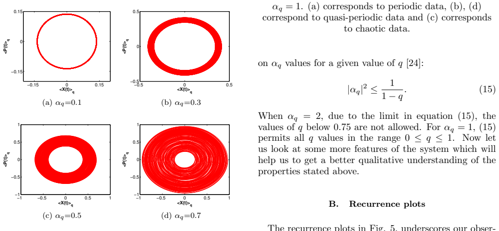
Starting from the q-deformed Hamiltonian $H_q = \frac{1}{2}(AA^\dagger + A^\dagger A)$ with $AA^\dagger - q^2 A^\dagger A = I$, the energy levels are $E_{q,n} = ([n] + q^{2n})/2$, with $[n] = (1-q^{2n})/(1-q^2)$. Because $[n]$ grows non-linearly with $n$, the spectrum is not equally spaced, unlike the ordinary oscillator. The paper shows that for coherent states $|\alpha\rangle_q$, the expectation values $\langle X(t)\rangle_q$ and $\langle P(t)\rangle_q$, computed from the time-evolved state in Eq. (10), are periodic for $q \lesssim 0.1$ (at $\alpha_q = 1$), quasi-periodic for $0.1 < q \lesssim 0.2$ and again near $q \to 1$, and chaotic for roughly $0.2 < q < 0.99$, with the chaotic window widening as $\alpha_q$ grows. Positive largest Lyapunov exponents and exponential first-return-time distributions confirm the chaotic classification.
Load-bearing premise
The calculation of every time series and every Lyapunov exponent rests on the time-evolved coherent state in Eq. (10); if the phase factor in that expression does not follow from the Hamiltonian (1), the computed regime boundaries are not reliable.
Editorial extensions
If this is right
- Chaos in a quantum system can be diagnosed from expectation-value time series of just two observables, without needing a classical or semiclassical limit.
- The regime map in Fig. 10 gives a parameter-by-parameter recipe: for fixed $\alpha_q$, sweeping $q$ moves the system through periodic, quasi-periodic, chaotic, and back toward quasi-periodic and periodic phases.
- Positive Lyapunov exponents in the chaotic band imply exponential divergence of nearby initial coherent states, so the deformation parameter controls sensitivity to initial conditions.
- Because the chaotic range widens with $\alpha_q$, larger coherent amplitudes at fixed deformation are more chaotic, while strong deformation restores order.
- The same diagnostic toolbox can be applied to other deformed algebras to test whether the periodic-to-chaotic regime sequence is universal.
Reading between the lines
- A direct consequence of the paper's own Eqs. (3) and (9) is that $E_{q,n} = 1/2 + q^2[n]/2$, so the phase factor in Eq. (10) would read $e^{-it/2} e^{-it q^2[n]/2}$. Recomputing the time series with this factor would test whether the regime boundaries in Fig. 10 move.
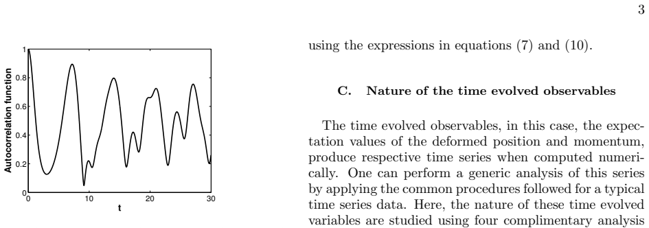
- The autocorrelation decay in Fig. 2 suggests a quantum-information probe: in the chaotic band, the fidelity of the deformed coherent state should decay irregularly, and quantifying that decay could give a state-based signature of the transition.
- Because the chaotic range depends on $\alpha_q$, the system is a tunable source of complex time series; engineering the deformation could serve as a controlled testbed for randomness generation or for time-series classification methods.
Signed reviews
Editorial analysis
A structured set of objections, weighed in public.
Referee Report
Summary. The manuscript studies the q-deformed harmonic oscillator with Hamiltonian H_q = (AA† + A†A)/2 and deformed commutation relation AA† − q^2 A†A = I. It constructs a q-deformed coherent state, derives the time-evolved expectation values ⟨X(t)⟩_q and ⟨P(t)⟩_q, and classifies their time series as periodic, quasi-periodic, or chaotic on the basis of recurrence plots, power spectra, first-return-time distributions, and Lyapunov exponents. The central claim is an explicit regime classification in the (q, α_q) plane (Fig. 10), with positive largest Lyapunov exponents in the chaotic regions.
Significance. If the central claim were correct, the paper would be a useful extension of earlier expectation-value-based studies of quantum dynamics to a q-deformed oscillator, and the regime classification could interest the quantum-optics community. The manuscript is explicit about the time-evolution formulas and provides a concrete set of falsifiable predictions, which are strengths. However, the model's energy spectrum is not consistently defined, and, independently of that ambiguity, the point-spectrum unitary evolution of this bounded-observable system cannot produce positive Lyapunov exponents. The reported numerical diagnostics therefore do not support the claimed chaotic regimes, and the classification in Fig. 10 is not reliable.
major comments (3)
- [II A, Eqs. (1), (3), (7), (9), (10)] The energy spectrum is defined inconsistently. From Eq. (7), A†A|n⟩ = [n]|n⟩ and AA†|n⟩ = [n+1]|n⟩, so Eq. (1) gives E_n = ([n]+[n+1])/2 = [n] + q^{2n}/2 = (1+(1+q^2)[n])/2. The printed Eq. (3), ([n]+q^{2n})/2, does not follow from the Hamiltonian and its q→1 limit is (n+1)/2, not the stated E_n = n+1/2. The phase factor in Eq. (10), exp(−it/2)exp(−it[n](1+q^2)/2), corresponds to the former spectrum, not to the printed Eq. (3). Thus the manuscript uses two different spectra. If Eq. (3) is intended, Eq. (10) should contain exp(−it q^2[n]/2) instead of exp(−it(1+q^2)[n]/2); if Eq. (10) is intended, Eq. (3) must be corrected. All subsequent expressions, Eqs. (11)–(13), and all numerical results inherit this ambiguity, so this is a load-bearing inconsistency.
- [III E, Fig. 8; Eqs. (1), (5), (6)] Positive Lyapunov exponents are impossible for this model. For 0<q<1 the Hamiltonian has a pure point spectrum with eigenvalues accumulating at a finite value, and X and P defined in Eqs. (5)–(6) are bounded operators because A and A† are bounded (sup_n [n] = 1/(1−q^2)). Consequently ⟨X(t)⟩_q and ⟨P(t)⟩_q are absolutely convergent trigonometric series in the bounded frequency differences E_m−E_n, i.e., they are almost periodic functions. Almost periodic functions do not exhibit exponential separation of nearby trajectories, so the positive λ_max values reported in Sec. III E and Fig. 8 must be finite-time or reconstruction artifacts of the Rosenstein/Wolf algorithms, not genuine properties of the oscillator. This objection is independent of the spectrum ambiguity in the previous comment and invalidates the central claim of chaotic regimes.
- [II C 3 and III D] The first-return-time analysis is circular as evidence for chaos. The paper defines ergodic behavior through the exponential first-return-time distribution F_1(τ) = (1/τ)e^{−t/τ} and then uses the fact that certain time series fit this distribution as a verification of ergodicity and as support for chaos. This applies the same criterion both as definition and as confirmation. Moreover, exponential first-return statistics also occur for non-chaotic stochastic and multi-frequency quasi-periodic signals, so this diagnostic cannot compensate for the absence of genuine Lyapunov exponents.
minor comments (6)
- [Eqs. (12)–(13)] In the second terms of Eqs. (12) and (13), the power of |α_q| appears to be off by one factor: the A† contribution should carry α_q^* |α_q|^{2n} (equivalently α_q^{−1}|α_q|^{2n+2}) rather than α_q^{−1}|α_q|^{2n+1}.
- [Fig. 2 and Sec. III A] The caption of Fig. 2 specifies q = 0.95 and |α_q|^2 = 1, while Sec. III A discusses the autocorrelation function peaking at random intervals for α_q = 1 and q = 0.9; the caption and the text should be made consistent.
- [Abstract and Introduction] The abstract's claim that detailed analysis of chaotic quantum systems based on expectation values 'has not been reported in the literature' is overstated, because Refs. [6–8] and [31] already perform such analyses; the novelty should be stated as the extension to q-deformed systems.
- [Fig. 10] The regime diagram in Fig. 10 is presented as an 'approximate demarcation' but the text does not explain how the boundaries were determined, what the axes' scaling is, or how the diagram was constructed from the numerical diagnostics; this makes the central classification difficult to reproduce.
- [II A, Eq. (8) and Eq. (15)] The normalization of the q-deformed coherent state in Eq. (8) and the bound in Eq. (15) are cited from Ref. [24] but not derived; since the q-exponential does not satisfy e_q(x)e_q(−x)=1, the normalization convention should be stated explicitly.
- [III E, Fig. 9] The parameter choices for the Lyapunov computations (embedding dimension, delay, and tolerance) are not fully specified for all figures; Fig. 9 shows m = 4, 6, 8 but the delay and the length of the linear fitting region are not given, which is important because the positive exponents are likely numerical artifacts.
Circularity Check
No significant circularity: the paper's classification is based on standard time-series diagnostics applied to directly computed expectation values, not on a fitted parameter or a self-citation chain.
full rationale
The paper's central derivation is self-contained. The time series for the expectation values <X(t)>_q and <P(t)>_q are obtained directly from the q-deformed coherent state in Eq. (8) and the Hamiltonian in Eq. (1), with no free parameters fitted to the quantities being classified. The periodic/quasi-periodic/chaotic classification is not the prediction of a fitted model; it is a set of diagnostic tools (recurrence plots, power spectra, first-return-time distributions, and Lyapunov exponents) applied to the same numerically generated time series. The use of the exponential first-return-time distribution as a signature of ergodicity is a standard application of the Poincaré recurrence theorem, not a definitional equivalence: the exponential form is a theoretical expectation, and the data are tested against it. The self-citations [6,7,8] concern the methodology and are not load-bearing; the methods are described in the text and are standard tools. The concerns raised in the reviewer context about almost-periodicity of bounded observables under point-spectrum unitary evolution, and about the phase factor in Eq. (10), are mathematical or correctness objections rather than circularity objections: they do not show that any input is being relabeled as a prediction. Accordingly, no circular step can be identified and the score is set to zero.
Assumptions & free parameters
free parameters (5)
- Truncation order for infinite sums =
not stated
- Time step and total integration time =
not stated
- Recurrence plot threshold epsilon =
not stated
- Embedding dimension and delay for Rosenstein algorithm =
m=4,6,8 shown; not specified which is used
- First-return-time cell size =
less than or equal to 10^-3
assumptions (4)
- domain assumption The q-deformed commutation relation AA† - q^2 A†A = I (Eq. 2) defines the model.
- domain assumption The deformed coherent state is defined by the q-exponential (Eq. 8).
- domain assumption Positive largest Lyapunov exponent of the expectation-value time series is taken as a signature of chaos.
- domain assumption The dynamics of expectation values in a finite truncation approximates the infinite-dimensional system.
Cite this review
Pith. "Pith review of Dynamics of observables in a $q$-deformed harmonic oscillator." pith.science (2026). https://pith.science/paper/KHWITW7M
@misc{pith2026190801467,
  author       = {Pith},
  title        = {Pith review of: Dynamics of observables in a $q$-deformed harmonic oscillator},
  year         = {2026},
  howpublished = {\url{https://pith.science/paper/KHWITW7M}},
  note         = {Machine review of arXiv:1908.01467}
}
abstract
Chaos in classical systems has been studied in plenty over many years. Although the search for chaos in quantum systems has been an area of prominent research over the last few decades, the detailed analysis of many inherently chaotic quantum systems based on expectation values of dynamical variables has not been reported in the literature. In this paper, we extend the study of dynamical behaviour using expectation values of variables to a $q$-deformed harmonic oscillator. The system is found to be periodic, quasi-periodic or chaotic depending on the values of the deformation parameter $q$ and the deformed coherent amplitude $\alpha_{q}$, thus enabling us to explicitly classify the chaotic nature of the system on the basis of these parameters. The chaotic properties of the system are clearly illustrated through recurrence plots, power spectra, first-return-time distributions and Lyapunov exponents of the time series obtained for the expectation values of the dynamic variables.
Figures


Figures from the paper (5 more)


Reference graph
Works this paper leans on
-
[1]
Recurrence plots: Recurrence plot is defined as the graphical representa- tion of Ri,j = { 1, if ⃗ xi≈ ⃗ xj; 0, otherwise. i,j = 1, 2,...N, (14) where N is the number of data points under considera- tion and ⃗ xi≈ ⃗ xj refers to its equivalence within a desig- nated parameterϵ [26]. The simulation of this calculation produces an N×N matrix, whose elements ...
-
[2]
Power spectra We also utilize the power spectrum of the time series to understand the nature of the non-linear system better. The power spectra are easily obtained by the technique of fast Fourier transform of the time series. It is to be noted that in case of a chaotic series, the power spectrum displays “grassiness” with the spectrum also showing a decr...
-
[3]
First-return-time distributions: First-return-time distribution encompasses informa- tion about the recurrence of a small range of values over a large series of datapoints [6, 7]. We construct computational cells of suitable sizes and determine 4 the frequency of recurrence of datapoints within this cell. We compute the probability of recurrence and attem...
-
[4]
Lyapunov exponent The next parameter analysed in this study is the Lyapunov exponent. The Lyapunov exponent ( λ) describes the divergence from an initial trajectory, of an almost identical trajectory produced by an infinites- imal perturbation in the initial conditions. A positive Lyapunov exponent is indicative of chaos in the system, in which case the tr...
-
[5]
R. V. Jensen, Nature 355, 311 (1992)
work page 1992
- [6]
- [7]
-
[8]
E. G. Vergini, J. Phys. A: Math. Gen. 33, 4709 (2000)
work page 2000
Show all 35 references
-
[9]
Wilkinson, J
M. Wilkinson, J. Phys. A: Math. Gen. 21, 1173 (1988). 8
1988
-
[10]
Sudheesh, S
C. Sudheesh, S. Lakshmibala and V. Balakrishnan, Phys. Lett. A 373, 2814 (2009)
2009
-
[11]
Sudheesh, S
C. Sudheesh, S. Lakshmibala and V. Balakrishnan, Eu- rophys. Lett. 90, 50001 (2010)
2010
-
[12]
Shankar, S
A. Shankar, S. Lakshmibala and V. Balakrishnan, J. Phys B: At. Mol. Opt. 47, 215505 (2014)
2014
-
[13]
Q. Zeng, J. Ge, H. Luo and Y. Luo, Int. J. Theor. Phys 56, 2738 (2017)
2017
-
[14]
Dupuis and F
M. Dupuis and F. Girelli, Phys. Rev. D 90, 104037 (2014)
2014
-
[15]
A. M. Gavrilik, I. I. Kachurik and Y. A. Mishchenko, J. Phys. A: Math. Theor. 44, 475303 (2011)
2011
-
[16]
A. A. Altintas, F. Ozaydin, C. Yesilyurt, S. Bugu and M. Arik, Quantum Inf. Process. 13, 1035 (2014)
2014
-
[17]
Behnia, M
S. Behnia, M. Yahyavi and R. Habibpourbisafar, Chaos, Soliton. Fract. 104, 6 (2017)
2017
-
[18]
Algin and A
A. Algin and A. S. Arikan, J. Stat. Mech. 2017, 043105 (2017)
2017
-
[19]
Q. J. Zeng, Z. Cheng and J. H. Yuan, Eur. Phys. J. B 81, 275 (2011)
2011
-
[20]
Guha and P
A. Guha and P. K. Das, Physica A 495, 18 (2018)
2018
-
[21]
A. A. A. Marinho, F. A. Brito and C. Chesman, J. Phys 568, 012009 (2014)
2014
-
[22]
A. A. Marinho, F. A. Brito and C. Chesman, Physica A 411, 74 (2014)
2014
-
[23]
Batouli, M
J. Batouli, M. El Baz, and A. Maaouni, Phys. Lett. A 379, 1619 (2015)
2015
-
[24]
S. Dey, A. Fring, L. Gouba and P. G. Castro, Phys. Rev. D 87, 084033 (2013)
2013
-
[25]
Sivakumar, J
S. Sivakumar, J. Opt. B- Quantum S. O. 2, R61 (2000)
2000
-
[26]
Rcamier, M
J. Rcamier, M. Gorayeb, W. L. Mochn and J. L. Paz, Int. J. Theor. Phys. 47, 673 (2008)
2008
-
[27]
M. P. Jayakrishnan, S. Dey, M. Faizal and C. Sudheesh, Ann. Phys. 385, 584 (2017)
2017
-
[28]
V. V. Eremin and A. A. Meldianov, Theor. Math. Phys. 147, 709 (2006) 147
2006
-
[29]
Sudheesh, S
C. Sudheesh, S. Lakshmibala and V. Balakrishnan, Phys. Lett. A 329, 14 (2004)
2004
-
[30]
Marwan, M
N. Marwan, M. C. Romano, M. Thiel and J. Kurths, Phys. Rep. 438, 237 (2007)
2007
-
[31]
R. S. Dumont and P. Brumer, J. Chem. Phys. 88, 1481 (1988)
1988
-
[32]
Baxter, Bull
G. Baxter, Bull. Amer. Math. Soc. 66, 472 (1960)
1960
-
[33]
M. T. Rosenstein, J. J. Collins and C. J. De Luca, Phys- ica D 65, 117 (1993)
1993
-
[34]
A. Wolf, J. B. Swift, H. L. Swinney and J. A. Vastano, Physica D 16, 285 (1985)
1985
-
[35]
Buzek, J
V. Buzek, J. Mod. Optic. 38, 801 (1991)
1991
Reviewed August 14, 2026 · model on record in the stance chip above.
Discussion (0). Continue with ORCID to comment.