REVIEW 5 major objections 5 minor 37 references
Autoregressive-Model-Based Methods for Online Time Series Prediction with Missing Values: an Experimental Evaluation
T0 review · 5 major / 5 minor · reviewed 2026-08-14 · deepseek-v4-flash
Pith's one-line read For online autoregressive prediction with missing values, filling gaps with the model's own forecast is reliable and beats sampling-based methods.
desk verdict Useful benchmark, but the AERR baseline is biased and the headline imputation conclusion does not follow. read the letter →
The pith
A machine-rendered reading of the paper's core claim, the machinery that carries it, and where it could break.
The reading
What carries the argument
The mechanism under comparison is the missing-value handling strategy, wrapped around the AR model $X_t=\sum_{i=1}^{p}\alpha_i X_{t-i}+\epsilon_t$. The three imputation-based methods (YW, KF, OGD) fill each missing $y_t$ with the current prediction $\tilde{y}_t$ and then feed the completed sequence into their standard estimator: YW solves the Yule-Walker equations for the autocorrelation coefficients, KF runs the predict-update Kalman recursion on a state-space model whose hidden state is the AR coefficient vector, and OGD updates coefficients by gradient descent on the squared one-step loss. AERR, adapted from attribute-efficient ridge regression, samples from the past $p$ observations to form an unbiased gradient estimate and discards sampled missing values, keeping imputation out of the coefficient update; ARLS is an offline EM-style least-squares method that iterates coefficient estimation and missing-value imputation and serves as the baseline. The comparison is designed to isolate what prediction-filling imputation, versus sampling around missingness, buys in online AR forecasting.
What would settle it
Re-run the five methods on the same synthetic AR data and missing masks, but at each missing time $t$ score the imputation $\tilde{y}_t$ against the true value $y_t$ that was deleted; if AERR then matches or beats YW and KF, the paper's main conclusion that imputation is reliably effective would be contradicted.
Extended reading notes
Core claim
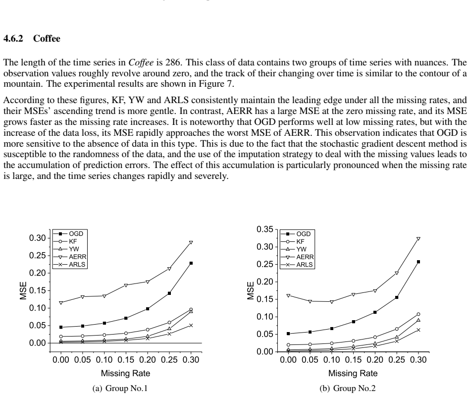
The paper's central claim is that, for AR-model time series with missing values in an online setting, imputation remains a simple but reliable and effective strategy. Concretely, the experiments show that missing-value-tolerant YW and KF—which replace each missing observation with their own one-step-ahead prediction before updating the model—keep MSE close to the offline ARLS baseline and to the white-noise variance of the generating process, while AERR, the sampling-based semi-imputation method, has the largest MSE under nearly all settings and on stock data reaches over ten times ARLS's error at a 30 percent missing rate. OGD also performs comparatively poorly and is sensitive to missing rates on real data. The claimed implication is that the imputation-absent, sampling-based route is not ideal in this online AR setting, and the practical choice among imputation methods should be driven by data properties: on some real series KF tolerates missingness better than YW, while YW struggles on non-seasonal or trending series and KF suffers when the noise is non-Gaussian.
Load-bearing premise
The comparison assumes that missing positions should not be counted as prediction errors; if the true values at those positions were scored against the imputed fill-ins, the imputation methods' apparent advantage could shrink or disappear.
Editorial extensions
If this is right
- Practitioners doing online AR forecasting with missing rates up to 30 percent can reasonably expect KF or YW with simple forecast-filling imputation to approach the accuracy of an offline baseline.
- Sampling-based imputation-absent methods such as AERR are unlikely to pay off in online AR settings unless their parameter-tuning and convergence issues are addressed.
- The best prediction order is the true AR order; increasing the fitted order beyond the generating order does not improve YW, KF, OGD, or ARLS, and it hurts AERR.
- Method choice should depend on the series: avoid YW for non-seasonal or strongly trending series, and avoid KF when the noise is clearly non-Gaussian.
- Longer training series shrink the performance gaps, particularly for the gradient-descent methods.
Reading between the lines
- A natural extension would test whether forecast-filling remains competitive when missingness is non-random, such as bursts of consecutive losses, since the paper only generates missing values independently with a fixed rate.
- A direct robustness check is to score imputed positions against the true values that the synthetic generator later reveals; the paper does not report this, and it could change the ranking.
- The results suggest a neighbouring question: whether the imputation advantage persists for ARMA or ARIMA models or for nonstationary series, which the experiments do not cover.
- The online AR benchmark could serve as a cheap testbed for neural-network-based missing-value methods, which the paper cites only as background.
Signed reviews
Editorial analysis
A structured set of objections, weighed in public.
Referee Report
Summary. The paper presents an experimental comparison of five methods for online prediction of autoregressive time series with missing values: Yule-Walker estimation (YW), Kalman filtering (KF), online gradient descent (OGD), attribute-efficient ridge regression (AERR), and an offline autoregressive least-squares imputation baseline (ARLS). The authors adapt each method to the online missing-value setting, describe them in Algorithms 1-5, and evaluate MSE under varying missing rates, series lengths, noise variances, AR coefficients, prediction model orders, and on four real datasets. The central conclusion, stated in Sections 4.7 and 5, is that imputation remains a simple, reliable, and effective strategy, whereas the sampling-based imputation-absent representative AERR performs worst overall and is especially sensitive to noise variance and rapidly changing series.
Significance. If the conclusions hold, the paper would provide practical guidance for choosing among online AR prediction methods under missing data, and it would support the common practice of prediction-filling imputation. The strengths of the paper are its systematic algorithmic exposition, the breadth of the experimental sweep (synthetic configurations plus four real datasets), and the inclusion of an offline baseline. However, the central claim is currently supported by a single imputation-absent representative whose implementation appears to have a biased gradient estimator, and several experimental choices (the MSE definition, the noise variance supplied to KF, and the absence of error bars) are not documented well enough to establish the reported rankings. The paper is a useful starting point for a comparison study, but the load-bearing evidence needs substantial clarification and re-analysis before the conclusions can be accepted.
major comments (5)
- [Section 3.4, Algorithm 4] The update rule in Algorithm 4 is not an unbiased stochastic gradient of the stated least-squares loss, contrary to the text's claim that the double sampling gives 'an unbiased estimation of the gradient' and that gamma is used 'to obtain unbiased estimations.' For p=1, let the observation be x and the missing indicator be m with P(m=1)=gamma. The first-stage estimator x_t equals x/(1-gamma) when observed and 0 when missing; the second-stage estimator phi equals alpha x/(1-gamma) - y when observed and 0 when missing. Because both estimators use the same missing indicator, E[phi x_t] = (1-gamma)(alpha x/(1-gamma) - y)(x/(1-gamma)) = alpha x^2/(1-gamma) - xy, whereas the true gradient is alpha x^2 - xy. The bias is alpha x^2 gamma/(1-gamma), which is nonzero for gamma>0 and alpha not equal to 0. The same correlation persists after marginalizing over the missing mask for p>1. Thus the poor MSE of AERR in Figures 1 and 6-9 may be an artifact of a biased update rather than evidence about sampling-based, imputation-absent methods. This is load-bearing because Section 4.7's conclusion that imputation is 'simple but reliable' depends on AERR being a fair representative of the imputation-absent class.
- [Section 4, MSE definition] The MSE definition, MSE(y1:T, ytilde1:T) = (1/T) sum_{t=1}^T (y_t - ytilde_t)^2, is undefined for missing positions because there is no observed y_t. The sentence that follows, saying y_i and ytilde_i denote the actual observation and prediction value, does not specify how missing indices enter the sum. If missing positions are included with y_t replaced by the imputed value, then for imputation-based methods such as YW, KF, and OGD the filled value is exactly their own prediction by construction, so those positions contribute zero error and mechanically favor imputation. If missing positions are excluded, the comparison is different. The paper must state exactly which convention is used, and the reported numbers in Tables/Figures should be recomputed or confirmed under that explicit convention.
- [Section 3.2 and Section 4.1] Algorithm 2 uses the observation noise variance sigma^2 inside the Kalman gain, G_t <- P_{t|t-1} H_t^T (H_t P_{t|t-1} H_t^T + sigma^2)^{-1}, and the synthetic experiments generate data with a known noise variance sigma^2 (the default theta in Section 4 sets sigma^2 = 0.32). If the experiments pass the true generating sigma^2 to KF, then KF receives oracle information about the noise that YW, OGD, and AERR do not have, which could explain why its MSE is so close to the offline ARLS baseline in Figure 1. The paper should disclose what value of sigma^2 was used for KF in each experiment, and ideally should include a variant in which sigma^2 is estimated online rather than given.
- [Section 4.1-4.6] All conclusions are based on point estimates of average MSE over 20 replications, but Figures 1-9 report no standard errors, confidence intervals, or significance tests. Some of the claimed separations are small, for example the gap between YW and KF in Figure 1, and Section 4.7 asserts that 'KF and YW have generally better performance' and that 'AERR is more sensitive to the noise variance.' Without measures of variability it is impossible to tell whether these orderings are stable across replications or particular to the reported runs. The paper should add error bars or intervals, or at least a table of mean and standard deviation for the main missing-rate experiment.
- [Section 4.6.1, AERR parameters] Algorithm 4 has mandatory parameters B, eta, and k, but the experimental section reports that k=10 was chosen by 'testing on several numbers' and gives no values for B or eta, no tuning grid, and no sensitivity analysis. Since AERR is the only imputation-absent method in the comparison, an under-tuned AERR would invalidate the conclusion that imputation-absent methods are inferior. The paper should report the full parameter settings used for AERR, describe the tuning procedure, and show how the results vary with B and eta.
minor comments (5)
- [Table 1] Rows 4 and 5 of Table 1 list the identical coefficient vector [0.1, 0.7, 0.7, 0.0, -0.5], so Figure 4(e) is a duplicate of Figure 4(d) rather than a fifth distinct setting. The intended fifth coefficient vector should be provided and the experiment re-run.
- [Figures 1-9] Many figure labels are corrupted into strings such as '/s48/s46/s48/s48' instead of readable text, making legends and axes difficult or impossible to interpret. These figures need to be regenerated with proper fonts and labels.
- [General reproducibility] No code, data, or parameter configuration files are provided. For an experimental evaluation paper, releasing the implementation and exact experimental scripts would substantially improve reproducibility and would also help verify the KF sigma^2 and MSE-convention questions raised above.
- [Notation and typos] The notation is inconsistent, with X_t used in Sections 2 and 3.3 while y_t is used elsewhere, and there are typos including 'Bayesain' (Section 3.2), 'overally' (Section 5), and 'F oundations' in reference [36]. Also, Section 4.5 introduces p_fit and p_gen but p_gen is not defined at that point; please define both explicitly.
- [References] References [4] and [5] appear to be the same paper by Anava, Hazan, and Zeevi cited in two different venues; this duplication should be cleaned up.
Circularity Check
No significant circularity: the paper is an experimental comparison, and its imputation-reliability conclusion is not forced by definitions or by a self-citation chain.
full rationale
This paper does not offer a formal derivation chain; it adapts five algorithms to an online AR prediction setting and compares them experimentally. The central conclusion that imputation is a simple but reliable strategy is supported by measured MSE comparisons over synthetic and real data, and it is not equivalent to any fitted parameter or definitional identity. The only potential self-citation is reference [34], used in Section 3.4 to justify the missing-rate correction in AERR's unbiased estimation; although the cited authors overlap with the present paper, this citation is an implementation detail rather than a step that reduces the paper's conclusion to its inputs, and the AERR estimator is externally checkable from Algorithm 4. Concerns about the exact handling of missing positions in the MSE computation or about the bias of AERR's gradient update are correctness and artifact concerns, not circularity, because the paper does not define its performance measure in terms of its own predictions in any quoted passage. No equation or fitted value is renamed as a prediction, and no uniqueness or ansatz is imported to force the experimental outcome. The finding is therefore no significant circularity, with score 0.
Assumptions & free parameters
free parameters (5)
- KF observation noise variance sigma^2 in synthetic experiments =
true generation value (e.g. 0.32 default)
- AERR sampling times k =
10
- AERR radius B and learning rate eta =
unspecified
- OGD learning rate eta =
varied per experiment, not reported as a table
- prediction model order p_fit =
5 default, 1 to 20 varied
assumptions (6)
- domain assumption Each synthetic time series is generated by a zero-mean stationary AR(p) process with fixed coefficients.
- domain assumption Missing values are missing completely at random, each position independently with a fixed probability.
- domain assumption MSE is computed over observed positions only.
- ad hoc to paper The adapted AERR is a fair representative of imputation-absent methods.
- domain assumption The Kalman filter's Gaussian noise assumption is appropriate for synthetic data and approximately for real data.
- standard math Yule-Walker equations give consistent AR coefficient estimates for stationary AR processes.
Cite this review
Pith. "Pith review of Autoregressive-Model-Based Methods for Online Time Series Prediction with Missing Values: an Experimental Evaluation." pith.science (2026). https://pith.science/paper/KQRCNTS3
@misc{pith2026190806729,
  author       = {Pith},
  title        = {Pith review of: Autoregressive-Model-Based Methods for Online Time Series Prediction with Missing Values: an Experimental Evaluation},
  year         = {2026},
  howpublished = {\url{https://pith.science/paper/KQRCNTS3}},
  note         = {Machine review of arXiv:1908.06729}
}
read the original abstract
Time series prediction with missing values is an important problem of time series analysis since complete data is usually hard to obtain in many real-world applications. To model the generation of time series, autoregressive (AR) model is a basic and widely used one, which assumes that each observation in the time series is a noisy linear combination of some previous observations along with a constant shift. To tackle the problem of prediction with missing values, a number of methods were proposed based on various data models. For real application scenarios, how do these methods perform over different types of time series with different levels of data missing remains to be investigated. In this paper, we focus on online methods for AR-model-based time series prediction with missing values. We adapted five mainstream methods to fit in such a scenario. We make detailed discussion on each of them by introducing their core ideas about how to estimate the AR coefficients and their different strategies to deal with missing values. We also present algorithmic implementations for better understanding. In order to comprehensively evaluate these methods and do the comparison, we conduct experiments with various configurations of relative parameters over both synthetic and real data. From the experimental results, we derived several noteworthy conclusions and shows that imputation is a simple but reliable strategy to handle missing values in online prediction tasks.
Figures


Figures from the paper (7 more)




Reference graph
Works this paper leans on
-
[1]
W. C.†, B. D. O. Anderson, M. Deistler, and A. Filler. Solutions of yule-walker equations for singular ar processes. Journal of Time, 32(5):531–538, 2011
work page 2011
-
[2]
H. Akaike. Fitting autoregressive models for prediction. Annals of the institute of Statistical Mathematics , 21(1):243–247, 1969
work page 1969
- [3]
- [4]
- [5]
-
[6]
J. D. Boyd, E. P. Kennelly, and P. Pistek. Estimation of eof expansion coefficients from incomplete data.Deep Sea Research Part I Oceanographic Research Papers, 41(10):1479–1488, 1994
work page 1994
-
[7]
Z. Che, S. Purushotham, K. Cho, D. Sontag, and Y . Liu. Recurrent neural networks for multivariate time series with missing values. 2016
work page 2016
-
[8]
M. K. Choong, M. Charbit, and H. Yan. Autoregressive-model-based missing value estimation for dna microarray time series data. IEEE Transactions on Information Technology in Biomedicine A Publication of the IEEE Engineering in Medicine & Biology Society , 13(1):131–137, 2009
work page 2009
Show all 37 references
-
[9]
Cottrell and P
M. Cottrell and P. Letremy. Missing values : processing with the kohonen algorithm. arXiv: Statistics Theory , pages 489–496, 2007
2007
-
[10]
J. Ding, L. Han, and X. Chen. Time series AR modeling with missing observations based on the polynomial transformation. Elsevier Science Publishers B. V ., 2010. 21 A PREPRINT - AUGUST 28, 2019
2010
-
[11]
Dunsmuir and P
W. Dunsmuir and P. M. Robinson. Estimation of time series models in the presence of missing data. Journal of the American Statistical Association , 76(375):560–568, 1981
1981
-
[12]
Earnest, M
A. Earnest, M. I. Chen, D. Ng, and L. Y . Sin. Using autoregressive integrated moving average (arima) models to predict and monitor the number of beds occupied during a sars outbreak in a tertiary hospital in singapore. BMC Health Services Research, 5(1):36, 2005
2005
-
[13]
G. Eshel. The yule walker equations for the ar coefficients. Internet resource, 2:68–73, 2003
2003
-
[14]
I. H. GRANT. Recursive least squares. Teaching Statistics, 9(1):15–18, 1987
1987
-
[15]
Hallin and J
M. Hallin and J. F. Ingenbleek. Nonstationary yule-walker equations. pages 189–195, 1983
1983
-
[16]
Hangos, R
K. Hangos, R. Lakner, and M. Gerzson. Intelligent Control Systems: An Introduction with Examples . Applied Optimization. Springer, 2001
2001
-
[17]
S. S. Haykin, S. S. Haykin, S. S. Haykin, and S. S. Haykin. Neural networks and learning machines , volume 3. Pearson Upper Saddle River, NJ, USA:, 2009
2009
-
[18]
Hazan and T
E. Hazan and T. Koren. Linear regression with limited observation. Computer Science, 2012
2012
-
[19]
A. E. Hoerl and R. W. Kennard. Ridge regression: Biased estimation for nonorthogonal problems. Technometrics, 12(1):55–67, 1970
1970
-
[20]
Honaker and G
J. Honaker and G. King. What to do about missing values in time-series cross-section data. American Journal of Political Science, 54(2):561–581, 2010
2010
-
[21]
R. H. Jones. Maximum likelihood fitting of arma models to time series with missing observations. Technometrics, 22(3):389–395, 1980
1980
-
[22]
R. E. Kalman et al. A new approach to linear filtering and prediction problems. Journal of basic Engineering , 82(1):35–45, 1960
1960
-
[23]
Karn and C
P. Karn and C. Partridge. Improving round-trip time estimates in reliable transport protocols. ACM SIGCOMM Computer Communication Review, 17(5):2–7, 1987
1987
-
[24]
Kirchgässner, J
G. Kirchgässner, J. Wolters, and U. Hassler. Autoregressive conditional heteroscedasticity.Introduction to Modern Time Series Analysis, pages 281–310, 2013
2013
-
[25]
T. Kohonen. Self-organizing maps. Springer Berlin Heidelberg, 1997
1997
-
[26]
Nocedal and S
J. Nocedal and S. J. Wright. Numerical Optimization. Springer, New York, 2nd edition, 2006
2006
-
[27]
I. Ojo. Autoregressive integrated moving average. Asian Journal of Mathematics and Statistics , 3(4):225–236, 2010
2010
-
[28]
R. W. Preisendorfer and C. D. Mobley. Principal component analysis in meteorology and oceanography. Develop- ments in Atmospheric Science , 17(50):55–72, 1988
1988
-
[29]
F. Scholz. Maximum likelihood estimation. Encyclopedia of statistical sciences , 1985
1985
-
[30]
Shang, L
Z. Shang, L. Zhang, S. Ma, B. Fang, and T. Zhang. Incomplete time series prediction using max-margin classifica- tion of data with absent features. Mathematical Problems in Engineering,2010,(2010-05-27), 2010(10):242–256, 2010
2010
-
[31]
Sorjamaa and A
A. Sorjamaa and A. Lendasse. Time series prediction as a problem of missing values: Application to estsp2007 and nn3 competition benchmarks. pages 2948–2953, 2007
2007
-
[32]
Tibshirani
R. Tibshirani. Regression shrinkage and selection via the lasso. Journal of the Royal Statistical Society. Series B (Methodological), pages 267–288, 1996
1996
-
[33]
S. Wang. Application of self-organising maps for data mining with incomplete data sets. Neural Computing and Applications, 12(1):42–48, 2003
2003
-
[34]
Y . Wei, H. Wang, S. Shi, H. Gao, and J. Li. Any-time methods for time-series prediction with missing observations. In G. Karypis and J. Zhang, editors, 2017 IEEE International Congress on Big Data, BigData Congress 2017, Honolulu, HI, USA, June 25-30, 2017 , pages 427–430. IE...
2017
-
[35]
Welch and G
G. Welch and G. Bishop. An Introduction to the Kalman Filter . University of North Carolina at Chapel Hill, 1995
1995
-
[36]
Ying and M
Y . Ying and M. Pontil. Online gradient descent learning algorithms.F oundations of Computational Mathematics, 8(5):561–596, 2008
2008
-
[37]
H. M. Zhang and P. Duhamel. On the methods for solving yule-walker equations. Signal Processing IEEE Transactions on, 40(12):2987–3000, 1992. 22
1992
Reviewed August 14, 2026 · model on record in the stance chip above.
Discussion (0). Continue with ORCID to comment.