A model of magnetic friction obeying the Dieterich--Ruina law in the steady state

Hisato Komatsu

REVIEW 3 major objections 4 minor 31 references

A model of magnetic friction obeying the Dieterich--Ruina law in the steady state

T0 review · 3 major / 4 minor · reviewed 2026-08-14 · deepseek-v4-flash

Challenge this review Re-run · record.json Download PDF Read on arXiv ↗ Review JSON

Pith's one-line read A two-lattice Ising model with antiferromagnetic edges produces steady-state magnetic friction obeying the Dieterich–Ruina law in the weak-force regime, for both smooth and rough surfaces.

desk verdict A modest numerical toy model with a genuine qualitative result—log-linear v–f in the low-force regime—but the quantitative DR claim rests on a fit to the same data, so it deserves review with a request for error bars and an independent barrier check. read the letter →

arxiv 1908.08887 v2 pith:KUIU6JUJ submitted 2019-08-23 cond-mat.stat-mech

Hisato Komatsu This is my paper · ORCID

classification cond-mat.stat-mech

keywords magneticfrictionDieterich–RuinalawIsingmodelthermalactivationKramersescapesteady-statesurfaceroughnessdepinningtransition

verification ladder T0 review T1 audit T2 compute T3 formal

The pith

A machine-rendered reading of the paper's core claim, the machinery that carries it, and where it could break.

The reading

This paper constructs a minimal statistical-mechanical model of magnetic friction: two adjacent square Ising lattices, the upper one pulled by a constant force, with the antiferromagnetic coupling between the lattices acting as a "potential barrier" that blocks sliding. The claim is that in the steady state, when the pulling force is weak, the friction force and sliding velocity satisfy the Dieterich–Ruina law $F = A\log v + B$, and that this holds for both a smooth and a rough sliding surface. The paper derives this from a Kramers-escape picture: the velocity is set by the probability of thermally hopping over a barrier whose height decreases linearly with applied force. If the claim is correct, it provides a controlled spin model in which a phenomenological law of rock and solid friction emerges from a simple microscopic interaction, without fine-tuning.

What carries the argument

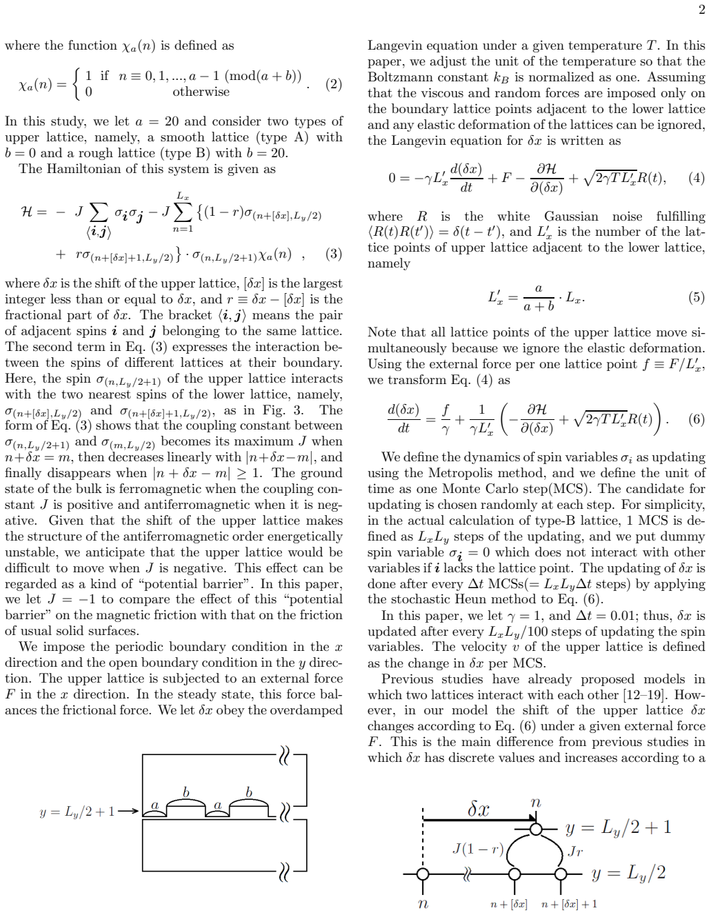
The engine of the argument is the effective potential $U(\delta x)$ generated by the antiferromagnetic coupling between the two lattices. Under an external force the total barrier height is $\bar U_{\max}-\bar U_{\min} = -\alpha F + L'_x u_0$, where $\alpha = \delta x_{\max} - \delta x_{\min}$ is the barrier width in lattice units and $u_0 = [U(\delta x_{\max})-U(\delta x_{\min})]/L'_x$ is the intrinsic barrier per boundary site. A Kramers-escape rate $v = \exp(c - (\text{barrier height})/T)$ then gives Eq. (12), and the equivalence to the Dieterich–Ruina law follows by reading $A = T/\alpha$ and $B = (L'_x u_0 - cT)/\alpha$. The simulations update the spins by Monte Carlo steps and move the upper lattice by the overdamped Langevin equation (6); the constants $c$, $\alpha$, and $u_0$ are extracted by least-squares fitting in the range $10^{-6} \le v \le 10^{-1}$.

What would settle it

Measure $v(f)$ for much smaller systems, say $L_x = 40$, at the same temperatures and fit Eq. (12); if the curves do not collapse when plotted against $F'$, or if the extracted $\alpha'$ deviates from $1/T$ with temperature while $T$ is changed, the Kramers-escape form is wrong. A more direct test is to sample the equilibrium distribution of $\delta x$ to compute $U(\delta x)$ and check whether the barrier height really drops linearly with $F$ with the fitted $\alpha$ and size-independent $u_0$.

Watch

Extended reading notes

Core claim

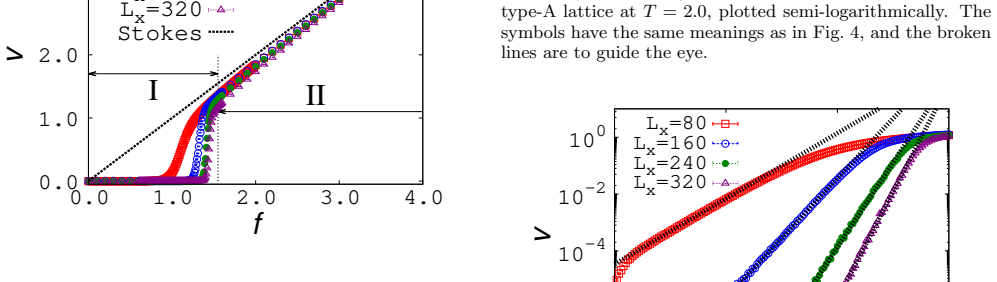
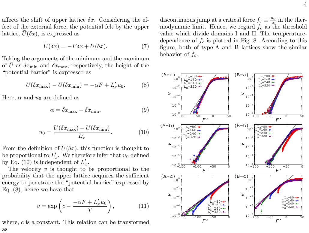
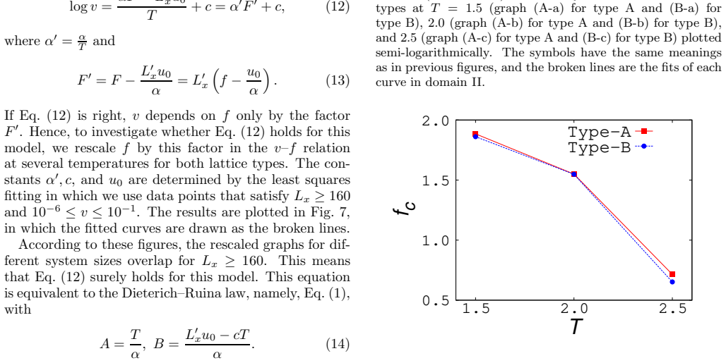
The central result is that the steady-state $v$–$f$ curve splits into two regimes. For large external force the sliding follows the Stokes law $v=f/\gamma$; for small force the motion is a thermally activated creep, and $\log v = \alpha' F' + c$ with $F' = L'_x (f - u_0/\alpha)$, which is exactly the steady-state Dieterich–Ruina law with $A=T/\alpha$ and $B=(L'_x u_0 - cT)/\alpha$. Numerical simulations at three temperatures and several system sizes show that $\log v$ plotted against the rescaled force $F'$ collapses onto a single master curve for the smooth (type A) and rough (type B) lattices, confirming Eq. (12) for $L_x \ge 160$. The threshold $f_c = u_0/\alpha$ remains nonzero even above the 2D Ising transition temperature $T_c \simeq 2.27$, so the barrier does not require long-range order.

Load-bearing premise

The argument assumes the sliding velocity is a thermally activated hop rate with a prefactor $c$ that does not depend on force or temperature, and that the intrinsic barrier $u_0$ per boundary site is independent of system size; if either fails, the log-linear law and the size collapse in Eq. (12) would break down.

Editorial extensions

If this is right

In the weak-force regime the model predicts a logarithmic friction law, so sliding speed changes by orders of magnitude while the force changes only linearly.
The threshold force $f_c = u_0/\alpha$ separates creep from Stokes sliding, and in the thermodynamic limit the velocity–force curve is expected to jump discontinuously at $f_c$.
The same logarithmic law appears for smooth and rough upper surfaces, so this version of the Dieterich–Ruina law does not depend on surface disorder.
Because $f_c$ stays nonzero above $T_c$, the barrier and the creep regime survive even when thermal fluctuations destroy long-range antiferromagnetic order.
The derived constants map the microscopic barrier shape ($\alpha$, $u_0$) onto the macroscopic Dieterich–Ruina coefficients $A$ and $B$, so the simulation gives a way to read off barrier parameters from friction data.

Reading between the lines

Editorial extensions of the paper, not claims the author makes directly.

The Kramers-escape derivation is generic: any surface interaction creating a barrier whose height falls linearly with applied force should give the same logarithmic creep law, so the mechanism may transfer to non-magnetic contacts.
The coefficient $B$ carries an explicit factor of system length $L'_x$, meaning the paper's Dieterich–Ruina parameters are not intrinsic material constants; a size-independent formulation would be needed to match experiments on finite contacts.
Only the steady-state law is shown; a natural extension is to drive the force or velocity in time and ask whether the full rate-and-state equations with a state variable emerge, not just the asymptotic logarithm.
The predicted jump at $f_c$ in the thermodynamic limit could be tested by finite-size scaling and by direct equilibrium measurement of $U(\delta x)$, which would independently verify the scaling form.

Share X Bluesky LinkedIn Reddit HN

Signed reviews

No signed human review yet.

Editorial analysis

A structured set of objections, weighed in public.

Desk editor's note, referee report, and a circularity audit.

Desk Editor's Note

read the letter

First thing to know: this is a small, earnest numerical study, and the part that matters is the qualitative log-linear v–f relation in the weak-force regime. That appears in the raw semi-log plots for both smooth and rough surfaces, before any fitting. The paper does something modest but genuinely new: it uses a force-controlled magnetic Ising model, unlike the velocity-fixed models of the earlier literature, and shows the steady-state velocity obeys the Dieterich–Ruina form over a range of forces.

What it does well: the model is clearly explained, the distinction between domains I and II is easy to see, and the comparison with earlier velocity-fixed models is fair. The collapse of the rescaled curves for Lx >= 160 is at least suggestive that a single-parameter scaling holds. The final section honestly concedes that B in Eq. (14) depends on L'_x, so the analogy with the DR law is not complete.

The soft spot is the fitting. Equation (12) is verified by fitting all three constants (u0, alpha, c) to the same data over a selected velocity window (10^-6 to 10^-1, Lx >= 160), and then the collapse is shown. That is a consistency check, not an independent prediction. The derivation of Eq. (11) treats the Kramers prefactor c as a constant and the barrier as strictly linear in f; the exact tilted periodic potential would give a prefactor that depends on f and a barrier that becomes nonlinear near threshold. So the mechanism is plausible but not nailed down. Also, the paper says error bars were collected over 96 trials but none are plotted, which makes the fit's stability hard to judge.

Are those fatal? No. For a toy model, the qualitative result stands on the raw data. The quantitative constants should be treated as effective parameters, not measured barrier properties. The paper itself flags the main mismatch with real DR friction.

Who is this for? People interested in microscopic foundations of rate-and-state friction, or in toy models that produce logarithmic velocity dependence from activation. It would be a useful entry in a reading group discussion about when a collapse actually confirms a mechanism. I'd send it to review; a referee should ask for error bars and an independent measurement of U(delta x) to check whether alpha and u0 match the fits, but the core observation is legitimate.

Referee Report

3 major / 4 minor

Summary. The paper introduces a lattice model of magnetic friction in which two Ising square lattices interact across a sliding boundary, with the upper lattice driven by an external force and relaxed by an overdamped Langevin dynamics plus Monte Carlo spin updates. The central claim is that in the weak-force regime (domain I) the steady-state velocity satisfies log v = alpha' F' + c, Eq. (12), which the authors identify with the Dieterich-Ruina law F = A log v + B, Eq. (1), and that this relation holds for both a smooth (type A) and a rough (type B) upper surface. The evidence consists of semi-logarithmic velocity-force plots at three temperatures and several system sizes, followed by a rescaling of the force axis using constants alpha', c, and u0 obtained by least-squares fitting, which produces the apparent collapse shown in Fig. 7. The paper also reports a force threshold fc and discusses the relation of the result to depinning and to the standard empirical friction law, acknowledging in Sec. IV that the coefficient B in Eq. (14) depends on the system size L'_x.

Significance. If the main claim is fully supported, the paper would provide a minimal, transparent magnetic lattice model that reproduces a Dieterich-Ruina-type steady-state velocity-force relation, including robustness to surface roughness and persistence above the equilibrium critical temperature. The simulation protocol is clearly specified, multiple system sizes are compared, and the smooth-versus-rough comparison is a genuine strength. The raw semi-logarithmic data do visually support a log-linear relation in domain I, and the collapse across Lx >= 160 is suggestive. However, the quantitative verification currently rests on fitting the same three constants that define the rescaling, and the connection to the standard Dieterich-Ruina law is weakened by the size-dependent offset B. The potential value of the model is real, but the paper needs an independent test of the assumed Kramers mechanism and a more careful statement of what exactly is meant by 'obeying the Dieterich-Ruina law.'

major comments (3)

[§III, Eq. (11)] The derivation of Eq. (11) assumes a Kramers escape form v = exp(c - (-alpha F + L'_x u0)/T) with a constant prefactor c, a constant activation length alpha, and a barrier offset u0 that is independent of L'_x. For an overdamped particle in a tilted periodic potential, the exact Kramers prefactor depends on the curvatures at the tilted minimum and maximum and hence on F, and near the depinning threshold the barrier height is not strictly linear in F. The paper does not measure U(delta x) directly, nor does it measure escape statistics independently. Since alpha', c, and u0 are fitted to the simulation data, the collapse in Fig. 7 is a post-fit consistency check rather than a parameter-free test of the mechanism. The load-bearing missing piece is an independent check: measure U(delta x) and the escape dynamics directly, and verify that the fitted alpha and u0 coincide with the measured barrier slope and offset.
[§III, fitting procedure before Fig. 7] The constants alpha', c, and u0 are determined by least-squares fitting using data points that satisfy Lx >= 160 and 10^-6 <= v <= 10^-1, and the same fitted values are then used to define the abscissa F' in the rescaled plots. The fitting window itself is chosen after inspecting the data, and no uncertainties or goodness-of-fit measures are reported. This makes the claimed collapse in Fig. 7 a post-hoc consistency check, not a validation of Eq. (12). The paper should report parameter uncertainties, show error bars or residual plots, and perform an out-of-sample test, for example fitting on one subset of system sizes or velocity ranges and predicting the rest, to demonstrate that the log-linear form is not simply absorbing a slowly varying prefactor through the fitted constants.
[§III-IV, Eq. (14)] Even if Eq. (12) holds, the paper's identification with the Dieterich-Ruina law, Eq. (1), is incomplete because the coefficient B in Eq. (14) depends on L'_x, whereas in the standard steady-state law A and B are constants for a given interface. The concluding section acknowledges this point, but the abstract and introduction state without qualification that the model 'obeys the Dieterich-Ruina law.' The claims should be restricted to a generalized DR-like logarithmic velocity dependence with a size-dependent offset, or the paper should argue explicitly why a size-dependent B is an acceptable generalization within the intended scope.

minor comments (4)

[Abstract and Introduction] The phrase 'the the velocity' appears in the abstract and in Sec. I; this should be corrected to 'the velocity.'
[Fig. 7 caption] The caption says 'the broken lines are the fits of each curve in domain II,' but the text describes the fits as being made in domain I (the DR-like regime); the caption should be corrected to avoid this contradiction.
[Sec. III, simulation paragraph] The text states that data are obtained 'with error bars,' but no error bars are visible in Figs. 4-7. The authors should either plot error bars or state in the captions that they are smaller than the symbol size, so that the scatter visible in the semi-logarithmic plots can be interpreted correctly.
[Sec. III, Fig. 8] The definition of the threshold fc = u0/alpha is somewhat ambiguous because u0 and alpha are fitted quantities; the paper should state whether the plotted fc values and their temperature dependence are derived from the same fits as in Fig. 7, and how the statistical uncertainty in fc is estimated.

Circularity Check

1 steps flagged · score 6.0 of 10

Eq. (12) is Eq. (11) rewritten with three constants fitted to the same data; the collapse in Fig. 7 is a post-fit consistency check, so the Dieterich–Ruina claim is partly circular.

fitted input called prediction [Sec. III, paragraph after Eq. (13) and Fig. 7]
"The constants α′, c , and u0 are determined by the least squares ﬁtting in which we use data points that satisfy Lx ≥ 160 and 10−6 ≤ v ≤ 10−1. The results are plotted in Fig. 7, in which the ﬁtted curves are drawn as the broken lines. According to these ﬁgures, the rescaled graphs for different system sizes overlap for Lx ≥ 160. This means that Eq. (12) surely holds for this model."

Eq. (12), log v = α′F′ + c, is obtained from Eq. (11), v = exp(c − (−αF + L′_x u0)/T), by the definitions F′ = F − L′_x u0/α and α′ = α/T, so it has no independent content beyond the assumed Kramers form. The same v–f data are used both to fit α′, c, and u0 by least squares and to verify the collapse. The three fitted constants set the slope, intercept, and horizontal shift of the curves, so the overlap in Fig. 7 only demonstrates that the assumed form describes the fitted residuals; it is not a parameter-free confirmation of the Dieterich–Ruina law. The identification F = A log v + B with A = T/α follows algebraically, so the central claim reduces to fitting the assumed Arrhenius barrier law.

full rationale

The model and simulations are original and self-contained, and the roughly linear log v versus f behavior in domain I is a real empirical observation. However, the paper's central identification with the Dieterich–Ruina law rests on Eq. (11), a Kramers form whose constants are not derived from the Hamiltonian or from a direct measurement of U(δx). The paper then fits α′, c, and u0 by least squares to the same velocity data used to validate Eq. (12), and because Eq. (12) is an algebraic rearrangement of Eq. (11), the Fig. 7 collapse is a post-fit consistency check rather than an independent prediction. This matches the pattern of a fitted input being presented as confirmation. The paper's own Sec. IV concession that B in Eq. (14) depends on L′_x further weakens the claimed analogy, though that is an incompleteness rather than circularity. No load-bearing self-citation chain is present; the partial circularity is the fit-based validation of the central DR-law claim.

Assumptions & free parameters 3 free parameters · 4 assumptions · 0 invented entities

The central quantitative claim hangs on three fitted constants and on Arrhenius escape with a force-independent prefactor. No new microscopic entities are introduced.

free parameters (3)

u0 (barrier height per boundary site) = not reported; fitted to data
Defined in Eq. (10) and fitted by least squares to the v-f data; controls the threshold fc = u0/alpha.
alpha (activation length) = not reported; fitted as alpha' = alpha/T
Distance between potential minimum and maximum; enters the slope of log v versus F.
c (log prefactor) = not reported
Additive constant in Eq. (11), fitted to the data; encodes the prefactor of the Arrhenius rate.

assumptions (4)

domain assumption The velocity is proportional to exp(-(barrier height)/T) with a prefactor independent of F and T (Arrhenius/Kramers escape).
Used in Eq. (11) to derive the Dieterich-Ruina form; no derivation of the prefactor is given.
domain assumption The effective potential U(delta x) is proportional to L'_x, so u0 = (U(xmax)-U(xmin))/L'_x is independent of system size.
Stated after Eq. (10); required for the rescaling collapse across Lx.
domain assumption The overdamped Langevin equation with white noise describes the surface motion while spins equilibrate via Metropolis updates.
Model definition in Eq. (4); not derived from a more microscopic Hamiltonian.
domain assumption The two-domain classification and threshold fc are defined by the fitted potential rather than by a sharp phase transition.
fc = u0/alpha is introduced after the fit; its thermodynamic-limit discontinuity is assumed but not proven.

how reviews work

0 comments

Cite this review

Pith. "Pith review of A model of magnetic friction obeying the Dieterich--Ruina law in the steady state." pith.science (2026). https://pith.science/paper/KUIU6JUJ

@misc{pith2026190808887,
  author       = {Pith},
  title        = {Pith review of: A model of magnetic friction obeying the Dieterich--Ruina law in the steady state},
  year         = {2026},
  howpublished = {\url{https://pith.science/paper/KUIU6JUJ}},
  note         = {Machine review of arXiv:1908.08887}
}

read the original abstract

We propose a model of magnetic friction and investigate the relation between the frictional force and the relative velocity of surfaces in the steady state. The model comprises two square lattices adjacent to each other, the upper of which is subjected to an external force, and the magnetic interaction acts as a kind of "potential barrier" that prevents the upper lattice from moving. We consider two surface types for the upper lattice: smooth and rough. The behavior of this model is classified into two domains, which we refer to as domains I and II. In domain II, the external force is dominant compared with other forces, whereas in the domain I, the the velocity of the lattice is suppressed by the magnetic interaction and obeys the Dieterich--Ruina law. This characteristic property can be observed regardless of whether the surface is smooth or rough.

Figures

Figures reproduced from arXiv: 1908.08887 by the authors.

**Figure 2.** FIG. 2: Lattice shape: the upper lattice lacks [PITH_FULL_IMAGE:figures/full_fig_p002_2.png] view at source ↗

**Figure 5.** FIG. 5: (Color online)The [PITH_FULL_IMAGE:figures/full_fig_p003_5.png] view at source ↗

Figures from the paper (3 more)

**Figure 4.** Figure 4: FIG. 4: (Color online)The [PITH_FULL_IMAGE:figures/full_fig_p003_4.png]

**Figure 7.** Figure 7: FIG. 7: (Color online)Rescaled [PITH_FULL_IMAGE:figures/full_fig_p004_7.png]

**Figure 8.** Figure 8: FIG. 8: (Color online)The temperature-dependence of the [PITH_FULL_IMAGE:figures/full_fig_p004_8.png]

Discussion (0). Continue with ORCID to comment.

Reference graph

Works this paper leans on

31 extracted references · 30 canonical work pages

[1]

Popova and V

E. Popova and V. L. Popov, Friction 3, 183 (2015)

2015
[2]

Baumberger and C.Caroli, Adv

T. Baumberger and C.Caroli, Adv. in Phys. 55, 279 (2006)

work page 2006
[3]

Kawamura, T

H. Kawamura, T. Hatano, N. Kato, S. Biswas, and B. K. Chakrabarti, Rev. Mod. Phys. 84, 839 (2012)

work page 2012
[4]

C. Mak, C. Daly, and J. Krim, Thin Solid Films 253, 190 (1994)

work page 1994
[5]

A. Dayo, W. Alnasrallah, and J. Krim, Phys. Rev. Lett. 80, 1690 (1998)

work page 1998
[6]

Highland and J

M. Highland and J. Krim, Phys. Rev. Lett. 96, 226107 (2006)

work page 2006
[7]

Pierno, L

M. Pierno, L. Bruschi, G. Fois, G. Mistura, C. Boragno, F.B. de Mongeot, and U.Valbusa, Phys. Rev. Lett. 105, 016102 (2010)

work page 2010
[8]

Kisiel, E

M. Kisiel, E. Gnecco, U. Gysin, L. Marot, S. Rast, and E. Meyer, Nature Mater. 10, 119 (2011)

work page 2011

Show all 31 references

[9]

Wolter, Y

B. Wolter, Y. Yoshida, A. Kubetzka, S.-W. Hla, K. von Bergmann, and R. Wiesendanger, Phys. Rev. Lett. 109, 116102 (2012)

2012
[10]

X. Cai, J. Wang, J. Li, Q. Sun, and Y. Jia, Trib. Inter. 95, 419 (2016)

2016
[11]

Li and W

Y. Li and W. Guo, Phys. Rev. B. 97, 104302 (2018)

2018
[12]

Kadau, A

D. Kadau, A. Hucht, and D. E. Wolf, Phys. Rev. Lett. 101, 137205 (2008)

2008
[13]

Hucht, Phys

A. Hucht, Phys. Rev. E. 80, 061138 (2009)

2009
[14]

Angst, A

S. Angst, A. Hucht, and D. E. Wolf, Phys. Rev. E. 85, 051120 (2012)

2012
[15]

Hucht and S

A. Hucht and S. Angst, Europhys. Lett. 100, 20003 (2012)

2012
[16]

Igl´ oi, M

F. Igl´ oi, M. Pleimling, and L. Turban, Phys. Rev. E. 83, 041110 (2011)

2011
[17]

H. J. Hilhorst, J. Stat. Mech. P04009 (2011). 6

2011
[18]

Li and M

L. Li and M. Pleimling, Phys. Rev. E. 93, 042122 (2016)

2016
[19]

Sugimoto, Phys

K. Sugimoto, Phys. Rev. E 99, 052103 (2019)

2019
[20]

Fusco, D

C. Fusco, D. E. Wolf, and U. Nowak, Phys. Rev. B. 77, 174426 (2008)

2008
[21]

D´ emery and D

V. D´ emery and D. S. Dean, Phys. Rev. L. 104, 080601 (2010)

2010
[22]

M. P. Magiera, L. Brendel, D. E. Wolf, and U. Nowak, Europhys. Lett. 87, 26002 (2009)

2009
[23]

M. P. Magiera, L. Brendel, D. E. Wolf, and U. Nowak, Europhys. Lett. 95, 17010 (2011)

2011
[24]

M. P. Magiera, S. Angst, and A. Hucht, and D. E. Wolf, Phys. Rev. B. 84, 212301 (2011)

2011
[25]

Ruina, J

A. Ruina, J. Geophys. Res. 88, 10359 (1983)

1983
[26]

J. H. Dieterich, Tectonophysics 144, 127 (1987)

1987
[27]

J. H. Dieterich, and B. D. Kilgore, Pure and Appl. Geophys. 143, 283 (1994)

1994
[28]

Heslot, T

F. Heslot, T. Baumberger, B. Perrin, B. Caroli, and C. Caroli, Phys. Rev. E. 49, 4973 (1994)

1994
[29]

C. H. Scholz, Nature 391, 37 (1998)

1998
[30]

Jeudy, A

V. Jeudy, A. Mougin, S. Bustingorry, W. Savero Torres, J. Gorchon, A. B. Kolton, A. Lema ˆ ıtre, and J.-P. Jamet, Phys. Rev. L. 117, 057201 (2016)

2016
[31]

Diaz Pardo, W

R. Diaz Pardo, W. Savero Torres, A. B. Kolton, S. Bustingorry, and V. Jeudy, Phys. Rev. B. 95, 184434 (2017)

2017

Pith tools

Reviewed August 14, 2026 · model on record in the stance chip above.

[1] [1]

Popova and V

E. Popova and V. L. Popov, Friction 3, 183 (2015)

2015

[2] [2]

Baumberger and C.Caroli, Adv

T. Baumberger and C.Caroli, Adv. in Phys. 55, 279 (2006)

work page 2006

[3] [3]

Kawamura, T

H. Kawamura, T. Hatano, N. Kato, S. Biswas, and B. K. Chakrabarti, Rev. Mod. Phys. 84, 839 (2012)

work page 2012

[4] [4]

C. Mak, C. Daly, and J. Krim, Thin Solid Films 253, 190 (1994)

work page 1994

[5] [5]

A. Dayo, W. Alnasrallah, and J. Krim, Phys. Rev. Lett. 80, 1690 (1998)

work page 1998

[6] [6]

Highland and J

M. Highland and J. Krim, Phys. Rev. Lett. 96, 226107 (2006)

work page 2006

[7] [7]

Pierno, L

M. Pierno, L. Bruschi, G. Fois, G. Mistura, C. Boragno, F.B. de Mongeot, and U.Valbusa, Phys. Rev. Lett. 105, 016102 (2010)

work page 2010

[8] [8]

Kisiel, E

M. Kisiel, E. Gnecco, U. Gysin, L. Marot, S. Rast, and E. Meyer, Nature Mater. 10, 119 (2011)

work page 2011