REVIEW 2 major objections 4 minor 41 references
A Dissipativity Framework for Constructing Scaled Graphs
T0 review · 2 major / 4 minor · reviewed 2026-08-06 · deepseek-v4-flash
Pith's one-line read For normal LTI systems, the scaled graph—a nonlinear generalization of the Nyquist plot—can be computed exactly by intersecting LMI-certified disk and half-plane regions, and the same LMI framework gives tight over-approximations for…
desk verdict Solid LMI framework for scaled graphs with a clean LTI exactness result; the reset-system proof has a real gap in the limit argument. read the letter →
The pith
A machine-rendered reading of the paper's core claim, the machinery that carries it, and where it could break.
The reading
What carries the argument
The computed object is the scaled graph $SG_U(H)=\{\rho(u,y)e^{\pm j\theta(u,y)}: u\in U\setminus\{0\},\, y\in H(u)\}$, where $\rho=\|y\|/\|u\|$ and $\theta=\arccos(\langle u,y\rangle/(\|u\|\|y\|))$. The workhorse is the matrix family $\Pi(\sigma,\lambda_c,r)=\sigma\begin{bmatrix}1 & -\lambda_c\\ -\lambda_c & \lambda_c^2-r^2\end{bmatrix}$ with $\sigma\in\{\pm1\}$, which generates exactly the interior disks $(\sigma=-1)$ and their exteriors $(\sigma=+1)$ centered on the real axis, together with half-planes as limiting cases. Each $\Pi$ defines a quadratic supply rate, and Lemma 4 says the system satisfies the corresponding IQC exactly when the scaled graph lies inside $S(\Pi)$. Feasibility of the associated KYP-style LMI in the storage matrix $P$ then certifies the region, and intersecting all certified regions produces the over-approximation. The exactness proof is carried by the Beltrami-Klein map $f_{BK}(z)=\frac{(\bar z-j)(z-j)}{1+|z|^2}$, which sends hyperbolic geodesic arcs to Euclidean line segments, so that hyperbolic convexity becomes Euclidean convexity and supporting half-planes in the disk correspond precisely to disk and exterior regions in the complex plane.
What would settle it
For a normal stable controllable LTI system, compute the true scaled graph from the transfer-function spectrum by Theorem 8 and compare it with the L1/L2 intersection on a dense grid of real centers; any residual area outside the true graph refutes exactness. For a reset system, find a single input $u\in L_2$ whose trajectory does not converge to zero (for example, a well-posed non-Zeno trajectory with persistent resets); if such an input exists, the limit step leading to the soft IQC (49) fails and the over-approximation argument collapses.
Extended reading notes
Core claim
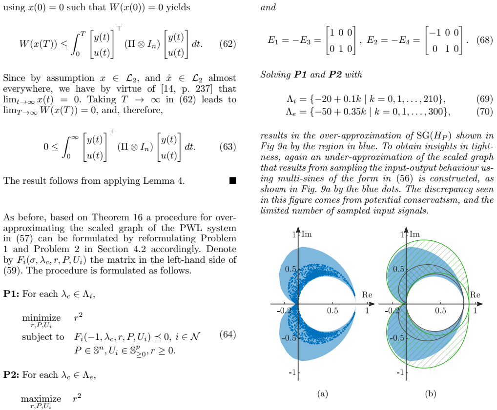
The paper's central claim is that scaled graphs do not have to be probed input-by-input: they can be built from the feasible set of a semidefinite program. Lemma 4 establishes that a stable system satisfies the IQC $\int_0^\infty \begin{bmatrix} y(t)\\ u(t) \end{bmatrix}^\top (\Pi\otimes I_n) \begin{bmatrix} y(t)\\ u(t) \end{bmatrix}dt\geq 0$ if and only if its scaled graph lies in the region $S(\Pi)=\{z\in\mathbb{C}: [z;\,1]^*\Pi[z;\,1]\geq 0\}$, which for $\det\Pi<0$ is a disk, the exterior of a disk, or a half-plane. Theorem 9 turns this into an LMI certificate: for an LTI system with Hurwitz $A$, existence of $P$ satisfying the KYP-style LMI implies the IQC, and under controllability all three statements—LMI feasibility, IQC, and scaled graph containment—are equivalent. The exactness theorem for normal LTI systems then uses the Beltrami-Klein mapping to convert the hyperbolic convex hull of the transfer-function spectrum into a Euclidean convex set, whose supporting half-planes correspond exactly to disk and exterior regions feasible for the LMIs; with $\Lambda_i=\Lambda_e=\mathbb{R}$ the intersection of all such regions is the closure of the scaled graph. For reset and piecewise-linear systems, Theorems 15 and 16 certify the same regions using jump and flow-set multipliers, giving over-approximations that the examples show are much tighter than the previous union-based approach.
Load-bearing premise
For all nonlinear, reset, and piecewise-linear results, the argument assumes that every admissible input produces square-integrable state and derivative trajectories, so the state decays to zero and the indefinite storage term can be discarded; for reset systems this decay step is applied to right-continuous trajectories with jumps, where the standard theorem does not directly apply.
Editorial extensions
If this is right
- For normal, stable, controllable LTI systems, the scaled graph can be computed exactly by solving the L1 and L2 LMI problems over all real centers, eliminating conservatism in that class.
- The same LMI machinery produces significantly tighter over-approximations for reset control systems than the previous union-based method, and extends to piecewise-linear systems.
- Feedback stability and L2-gain bounds for mixed interconnections (LTI with resets, resets with piecewise-linear systems) can be verified graphically through scaled-graph separation, with robustness margins read directly from the plots.
- Hard scaled graphs for unbounded systems such as integrators are obtained by the same procedure with the extra constraint $P\succeq 0$, so the framework covers systems outside $L_2$.
- The construction is not tied to continuous-time LTI structure and can be adapted to any system class with LTI-like state-space descriptions, including discrete-time, LPV, and Lur'e systems.
Reading between the lines
- A natural next test, not run in the paper, is whether the exactness theorem extends to non-normal LTI systems; comparing the L1/L2 intersection against the Beltrami-Klein hull of the full numerical range would show whether normality is essential.
- The exact LMI-intersection representation suggests an adaptive algorithm: instead of dense grids of centers $\lambda_c$, one can place new disks where the current over-approximation most exceeds a sampled under-approximation, achieving certified $\varepsilon$-tightness with far fewer LMI solves.
- The reset-system proof invokes a decay theorem for absolutely continuous functions on right-continuous trajectories with jumps; a dwell-time or jump-bound condition may be needed to make the soft scaled graph argument fully rigorous, and a counterexample input with persistent resets would settle it.
- Because separation of scaled graphs is a sufficient stability condition, exact computation for LTI components opens a loop-shaping design route: choose controller parameters so that the controller's scaled graph avoids the inverse scaled graph of the plant, with the LMI intersection as a fast graphical check.
Editorial analysis
A structured set of objections, weighed in public.
Referee Report
Summary. The manuscript proposes an LMI-based dissipativity framework for computing scaled graphs of dynamical systems. It first establishes a link between quadratic integral quadratic constraints of the form (13) and disk/half-plane regions in the complex plane (Lemma 4), then uses this to construct over-approximations of scaled graphs by intersecting the regions generated by feasible matrices. For normal LTI systems, Theorem 12 claims exactness of the intersection when all disk centers on the real line are used. The framework is extended to reset systems (Theorem 15) and piecewise linear systems (Theorem 16) by combining the LMI conditions with S-procedure arguments, and to hard scaled graphs by adding a positive-semidefinite storage constraint. The paper closes with numerical examples, including feedback interconnection tests based on a scaled-graph separation theorem.
Significance. If the results hold, the paper gives a practical convex route to scaled-graph construction for several system classes, and the exactness result for normal LTI systems is a genuinely novel contribution that goes beyond transfer-function-based constructions. The paper is self-contained, uses standard tools (KYP lemma, S-procedure, supporting hyperplane theorem), and does not fit free parameters to benchmark outputs. The comparison with the reset-system method of [35] suggests a substantial reduction of conservatism. However, the proof of the reset-system theorem contains a genuine gap in the passage from a finite-horizon dissipation inequality to the global IQC, so the nonlinear extension is not yet established as stated.
major comments (2)
- [Section 5.1, Theorem 15, Eqs. (48)-(49)] The proof invokes [14, p. 237] to conclude lim_{t→∞} x(t) = 0 from x, ẋ ∈ L2, and then takes T → ∞ in (48) to obtain the soft IQC (49). The cited result is for absolutely continuous functions, but reset trajectories in (42) are only right-continuous and piecewise absolutely continuous, with jumps at reset instants. For such signals, membership in L2 together with an L2 a.e. derivative does not force a limit at infinity: for example, f(t)=1 on intervals [n, n+n^{-2}] and f(t)=0 elsewhere satisfies f, f′ ∈ L2 with f′ = 0 a.e. but has no limit as t→∞. Therefore W(x(T)) in (48) need not vanish along reset trajectories, and the step from (48) to (49) is not justified. This is load-bearing because (49) is exactly the IQC used to apply Lemma 4 and conclude SG_U(H_R) ⊆ S(Π). The authors should either add a reset-aware convergence argument (e.g., summability of reset increments or a direct dissipation-based limit) or impose an additional assumption that guarantees lim_{t→∞} x(t) = 0 along all admissible reset trajectories.
- [Theorem 12, Section 4.3, proof around Eq. (36)] The proof of exactness applies Lemma 11, which assumes that the closed convex set has nonempty interior. However, f_BK(SG(H_L)_+) can be a curve segment with empty interior: for the first-order system in Remark 14 the scaled graph is a circle, whose image under the Beltrami-Klein map is a line segment. Thus the hypothesis of Lemma 11 is not verified for cases that the theorem is intended to cover. The conclusion of (36) is still true by the standard supporting-hyperplane theorem for general closed convex sets, so the argument is repairable, but as written the cited lemma does not support the claim.
minor comments (4)
- [Section 2.3] In the text introducing the Beltrami-Klein mapping, “maping” should be “mapping”.
- [Section 5.2] In the sentence “not limited to te systems considered,” “te” should be “the”.
- [Abstract and Remark 13] The abstract states that the approach “is shown to be exact for specific linear time-invariant systems,” but Theorem 12 establishes equality with the closure of the scaled graph and requires solving infinitely many LMIs (Λ_i = R and Λ_e = R). Remark 13 acknowledges this, but the abstract would benefit from the same qualification to avoid overstating the algorithmic exactness.
- [Example 2 and Figure 7] The comparison with the method of [35] would be more reproducible if the authors specified whether the same grid sets Λ_i and Λ_e and the same computational effort were used for both methods.
Circularity Check
No significant circularity: the exactness result rests on an external characterization (Pates' Theorem 8) and self-contained LMI/IQC equivalences; self-citations are contextual or benchmark comparisons only.
full rationale
I walked the derivation chain. The central over-approximation result (Theorem 5) is definitional in the benign sense that Π(H) is defined by IQCs and Lemma 4 proves SGU(H)⊂S(Π) iff the IQC holds; the scaled graph is defined independently through gains and phases in (1)-(3), while IQCs are defined through quadratic supply rates in (12)-(13), so the equivalence is a proved algebraic fact rather than a circular identification. The LTI procedure in Section 4 uses the KYP lemma (Theorem 9) to connect LMI feasibility to IQCs, and the exactness theorem (Theorem 12) invokes Pates' Theorem 8, an external result for normal LTI systems, to characterize the target scaled graph; it then shows that every supporting half-plane of the Beltrami-Klein image corresponds to a feasible Π in L1/L2, so the intersection of the LMI-generated regions collapses to the scaled graph. No parameter is fitted to match the predicted scaled graph; the grids Λi and Λe are computational sampling parameters, not degrees of freedom tuned to the output. The reset and piecewise-linear extensions (Theorems 15 and 16) are self-contained dissipation arguments, with [14, p.237] used only as a standard limit lemma. The self-citations present in the paper, such as [13], [34], [35], and [36], are used for background, for the benchmark comparison, or for the numerical example taken from [35, Example 1]; none carries a load-bearing premise that is unverified outside the present paper. A separate correctness concern exists in Theorem 15's passage from the finite-horizon inequality (48) to the soft IQC (49) via lim_{t→∞} x(t)=0 for reset trajectories that are only right-continuous piecewise absolutely continuous, because the cited Desoer-Vidyasagar result applies to absolutely continuous functions; that is a proof gap or mathematical-risk issue, not a circularity, and therefore does not affect the circularity score.
Assumptions & free parameters
free parameters (1)
- Finite grids Λi and Λe of disk centers λc =
e.g., (33a)-(33b), (34a)-(34b), (54)-(55), (69)-(70)
assumptions (5)
- domain assumption Theorem 8 of Pates [26]: for a normal, stable LTI system, SG(HL) = f^{-1}_BK(hull(f_BK(σ(HL))))
- standard math Kalman-Yakubovich-Popov lemma (Rantzer, 1996)
- standard math Supporting half-plane intersection (Lemma 11)
- domain assumption Trajectories of reset/PWL systems satisfy x, ẋ ∈ L2 for u∈U, implying lim x(t)=0
- domain assumption Well-posedness of reset system solutions with isolated resets and Carathéodory solutions for PWL systems
Cite this review
Pith. "Pith review of A Dissipativity Framework for Constructing Scaled Graphs." pith.science (2026). https://pith.science/paper/KWAO44UD
@misc{pith2026250708411,
  author       = {Pith},
  title        = {Pith review of: A Dissipativity Framework for Constructing Scaled Graphs},
  year         = {2026},
  howpublished = {\url{https://pith.science/paper/KWAO44UD}},
  note         = {Machine review of arXiv:2507.08411}
}
read the original abstract
Scaled relative graphs have been originally introduced in the context of convex optimization and have recently gained attention in the control systems community for the graphical analysis of nonlinear systems. Of particular interest in stability analysis of feedback systems is the scaled graph, a special case of the scaled relative graph. In many ways, scaled graphs can be seen as a generalization of the classical Nyquist plot for linear time-invariant systems, and facilitate a powerful graphical tool for analyzing nonlinear feedback systems. In their current formulation, however, scaled graphs require characterizing the input-output behaviour of a system for an uncountable number of inputs. This poses a practical bottleneck in obtaining the scaled graph of a nonlinear system, and currently limits its use. This paper presents a framework grounded in dissipativity for efficiently computing the scaled graph of several important classes of systems, including multivariable linear time-invariant systems, impulsive systems, and piecewise linear systems. The proposed approach leverages novel connections between linear matrix inequalities, integral quadratic constraints, and scaled graphs, and is shown to be exact for specific linear time-invariant systems. The results are accompanied by several examples illustrating the potential and effectiveness of the presented framework.
Figures


Figures from the paper (7 more)




Reference graph
Works this paper leans on
-
[35]
S. J. A. M. van den Eijnden, T. Chaffey, T. Oomen, and W. P. M. H. Heemels. Scaled graphs for reset control system analysis. European Journal of Control, 80:101050, November 2024
work page 2024
-
[1]
W. H. T. M. Aangenent, G. Witvoet, W. P. M. H. Heemels, M. J. G. van de Molengraft, and M. Steinbuch. Performance analysis of reset control systems. International Journal of Robust and Nonlinear Control , 20(11):1213–1233, 2010
work page 2010
-
[2]
E. Baron-Prada, A. Anta, and F. D¨ orfler. On decentralized stability conditions using scaled relative graphs. IEEE Control Systems Letters , 2025
work page 2025
-
[3]
E. Baron-Prada, A. Anta, A. Padoan, and F. D¨ orfler. Mixed Small Gain and Phase Theorem: A new view using Scale Relative Graphs, March 2025. arXiv:2503.13367 [math]
arXiv 2025
-
[4]
E. Baron-Prada, A. Anta, A. Padoan, and F. D¨ orfler. Stability results for MIMO LTI systems via Scaled Relative Graphs, March 2025. arXiv:2503.13583 [eess]
arXiv 2025
-
[5]
Boyd and L
S. Boyd and L. Vandenberghe. Convex Optimization . Cambridge University Press, 2004
2004
-
[6]
T. Chaffey. A rolled-off passivity theorem. Systems & Control Letters, 162:105198, 2022
work page 2022
-
[7]
T. Chaffey, F. Forni, and R. Sepulchre. Scaled relative graphs for system analysis. In 2021 60th IEEE Conference on Decision and Control (CDC), pages 3166–3172. IEEE, 2021
work page 2021
Show all 41 references
-
[8]
Chaffey, F
T. Chaffey, F. Forni, and R. Sepulchre. Loop Shaping with Scaled Relative Graphs, August 2022. arXiv:2208.04880 [cs, eess]
2022 arXiv
-
[9]
Chaffey, F
T. Chaffey, F. Forni, and R. Sepulchre. Graphical nonlinear system analysis. IEEE Transactions on Automatic Control , 68(10):6067–6081, 2023
2023
-
[10]
Chaffey and A
T. Chaffey and A. Padoan. Circuit model reduction with scaled relative graphs. In 2022 IEEE 61st Conference on Decision and Control (CDC) , pages 6530–6535, 2022
2022
-
[11]
C. Chen, T. Chaffey, and R. Sepulchre. Graphical dominance analysis for linear systems: A frequency-domain approach,
-
[12]
C. Chen, S. Z. Khong, and R. Sepulchre. Soft and hard scaled relative graphs for nonlinear feedback stability, 2025. arXiv:2504.14407 [eess]
2025 arXiv
-
[13]
de Groot, T
T. de Groot, T. Oomen, and S. J. A. M. van den Eijnden. Exploiting structure in mimo scaled graph analysis, 2025. arXiv:2504.10135 [eess.SY]
2025 arXiv
-
[14]
C. A. Desoer and M. Vidyasagar. Feedback Systems. Society for Industrial and Applied Mathematics, 2009
2009
-
[15]
R. A. Freeman. On the Role of Well-Posedness in Homotopy Methods for the Stability Analysis of Nonlinear Feedback Systems. In Zhong-Ping Jiang, Christophe Prieur, and Alessandro Astolfi, editors, Trends in Nonlinear and Adaptive Control: A Tribute to Laurent Praly for his 65th...
2022
-
[16]
Goebel, R
R. Goebel, R. G. Sanfelice, and A. R. Teel.Hybrid Dynamical Systems: Modeling, Stability, and Robustness . Princeton University Press, 2012. 15 (a) (b) (c) Fig. 11. Over-approximations of the hard scaled graphs in blue and the soft scaled graphs in the hatched black regions. (...
2012
-
[17]
W. M. Griggs, B. D. Anderson, A. Lanzon, and M. C. Rotkowitz. Interconnections of nonlinear systems with “mixed” small gain and passivity properties and associated input–output stability results. Systems & Control Letters , 58(4):289–295, 2009
2009
-
[18]
Hespanha
J.P. Hespanha. Linear Systems Theory: Second Edition . Princeton University Press, 2018
2018
-
[19]
Huang, E
X. Huang, E. K. Ryu, and W. Yin. Scaled Relative Graph of Normal Matrices, January 2020. arXiv:2001.02061 [cs, math]
2020 arXiv
-
[20]
Iwasaki and S
T. Iwasaki and S. Hara. Generalized KYP lemma: unified frequency domain inequalities with design applications.IEEE Transactions on Automatic Control , 50(1):41–59, January 2005
2005
-
[21]
Iwasaki and S
T. Iwasaki and S. Hara. Generalized kyp lemma: unified frequency domain inequalities with design applications.IEEE Transactions on Automatic Control, 50(1):41–59, 2005
2005
-
[22]
J. P. J. Krebbekx, R. T´ oth, and A. Das. SRG Analysis of Lur’e Systems and the Generalized Circle Criterion, November 2024. arXiv:2411.18318 [eess]
2024 arXiv
-
[23]
R. I. Leine and N. van de Wouw. Non-smooth Dynamical Systems, pages 59–77. Springer Berlin Heidelberg, Berlin, Heidelberg, 2008
2008
-
[24]
Megretski and A
A. Megretski and A. Rantzer. System analysis via integral quadratic constraints. IEEE Transactions on Automatic Control, 42(6):819–830, June 1997. Number: 6 Conference Name: IEEE Transactions on Automatic Control
1997
-
[25]
T. Needham. Visual Complex Analysis . Oxford University Press, Oxford, 1997
1997
-
[26]
R. Pates. The Scaled Relative Graph of a Linear Operator, August 2021. arXiv:2106.05650 [math]
2021 arXiv
-
[27]
J. Quan, B. Evens, R. Sepulchre, and P. Patrinos. Scaled Relative Graphs for Nonmonotone Operators with Applications in Circuit Theory, November 2024. arXiv:2411.17419 [math]
2024
-
[28]
A. Rantzer. On the Kalman—Yakubovich—Popov lemma. Systems & Control Letters , 28(1):7–10, June 1996
1996
-
[29]
E. K. Ryu, R. Hannah, and W. Yin. Scaled relative graphs: Nonexpansive operators via 2d euclidean geometry. Mathematical Programming, 194(1):569–619, 2022
2022
-
[30]
Samanipour and H
P. Samanipour and H. A. Poonawala. Stability analysis and controller synthesis using single-hidden-layer relu neural networks. IEEE Transactions on Automatic Control , 69(1):202–213, 2024
2024
-
[31]
Scherer and S
C. Scherer and S. Weiland. Linear Matrix Inequalities in Control. 2015
2015
-
[32]
K. Shi, N. Nikooienejad, I. R. Petersen, and S. O. R. Moheimani. Negative imaginary control using hybrid integrator-gain systems: Application to mems nanopositioner. IEEE Transactions on Control Systems Technology, 32(3):718–730, 2024
2024
-
[33]
R. T´ oth. Modeling and identification of linear parameter- varying systems , volume 403. Springer, 2010
2010
-
[34]
S. J. A. M. Van Den Eijnden and T. Chaffey. Characterizing nonlinear systems with mixed input-output properties through dissipation inequalities. In 2024 IEEE 63rd Conference on Decision and Control (CDC) , pages 5138– 5143, 2024
2024
-
[36]
S. J. A. M. Van Den Eijnden, M. F. Heertjes, W. P. M. H. Heemels, and H. Nijmeijer. Hybrid Integrator-Gain Systems: A Remedy for Overshoot Limitations in Linear Control? IEEE Control Systems Letters , 4(4):1042–1047, October 2020. Number: 4
2020
-
[37]
Van Der Schaft
A. Van Der Schaft. L2-Gain and Passivity Techniques in Nonlinear Control . Communications and Control Engineering. Springer International Publishing, Cham, 2017
2017
-
[38]
J. C. Willems. Dissipative dynamical systems. European Journal of Control , 13(2):134–151, 2007
2007
-
[39]
Zaccarian, D
L. Zaccarian, D. Nesic, and A. R. Teel. First order reset elements and the Clegg integrator revisited. In Proceedings of the 2005, American Control Conference, 2005., pages 563– 568, Portland, OR, USA, 2005. IEEE
2005
-
[40]
Zhang, M
X. Zhang, M. B. Kaczmarek, and S. Hassan Hosseinnia. Frequency response analysis for reset control systems: Application to predict precision of motion systems. Control Engineering Practice, 152:106063, 2024. 16
2024
-
[2025]
arXiv:2504.14394 [eess]
Reviewed August 6, 2026 · model on record in the stance chip above.
Discussion (0). Continue with ORCID to comment.