REVIEW 3 major objections 5 minor 76 references
HI bias parameters are not independent: a learned mapping from halo-occupation physics yields tight, non-Gaussian priors for 21 cm cosmology.
Reviewed by Pith at T0; open to challenge. T0 means a machine referee read the full paper against a public rubric. the ladder, T0–T4 →
T0 review · deepseek-v4-flash
2026-08-02 02:46 UTC pith:L7UK6OIX
load-bearing objection A credible proof-of-concept for HI simulation-based EFT priors; the central claim of a structured HOD-to-bias mapping is robust, but the bias-extraction step needs more validation before the tight priors are taken at face value. the 3 major comments →
Simulation-Based Priors for HI Bias from Halo Occupation Physics
The pith
A machine-rendered reading of the paper's core claim, the machinery that carries it, and where it could break.
Core claim
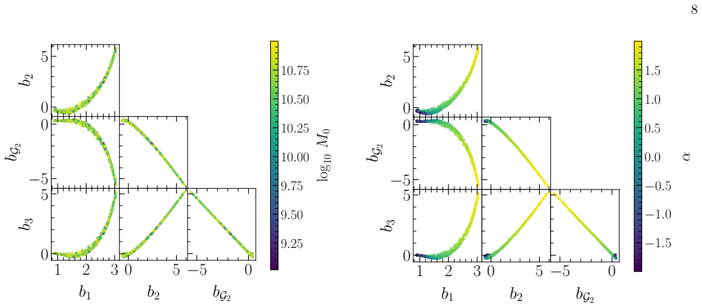
On the paper's own terms, the central discovery is that the HOD-to-bias relation for neutral hydrogen is not a loose cloud but a thin, curved manifold: across an ensemble of 2,000 HOD realizations per redshift, the four EFT bias parameters occupy a correlated, non-Gaussian region of parameter space, and the high-mass slope α acts as the main organizing direction. When a conditional normalizing flow is trained on paired HOD/bias samples, it reproduces this structure and can be sampled to yield simulation-based priors. Propagating a CHORD-like 21 cm power-spectrum measurement on nonlinear scales through the flow gives priors on (b1,b2,bG2,b3) that are dramatically tighter than flat priors, mos
What carries the argument
The central object is the conditional density p(θ_EFT | θ_HOD), the distribution of the EFT bias parameters given the four parameters (M0, Mmin, α, β) of a simplified HI halo-occupation model. The paper estimates it with a conditional normalizing flow—an invertible neural map from a Gaussian base to the target density, conditioned on the HOD parameters—trained by maximum likelihood on paired samples generated from simulations. This flow does the work of encoding the curved, correlated, non-Gaussian support of the bias manifold and providing a sampleable prior; without it the structure visible in the HOD scan could not be turned into a usable prior.
Load-bearing premise
The load-bearing premise is that the fitted k→0 limits of the transfer functions—obtained by extrapolating smooth polynomial fits over a quasi-linear k range—give unbiased values of (b1,b2,bG2,b3); if the true k-dependence is not captured by those forms, every bias estimate and the prior built from them is systematically wrong.
What would settle it
Take a single set of HOD realizations and infer the bias parameters with a finer mesh and a more complete operator basis (e.g., including all independent third-order operators); if the extracted (b1,b2,bG2,b3) move by more than the width of the flow prior, the prior is not robust. Alternatively, increase the simulation volume and check whether the offsets between the two simulation suites shrink; if they persist, the simulation dependence is a genuine property, not finite-volume noise.
If this is right
- Replacing broad, independent flat priors on HI bias parameters with the flow-based prior significantly tightens EFT-parameter posteriors in full-shape 21 cm analyses; at z=3 the covariance volume shrinks by roughly two orders of magnitude as observing time grows from 100 to 1000 days.
- The learned conditional density can be used in two ways: directly as a simulation-based prior, or as a map that converts external or nonlinear-scale constraints on HOD parameters into an induced prior on EFT bias parameters.
- The mapping is organized mainly by the high-mass slope α; M0 has almost no effect on the deterministic overdensity field, while Mmin and β mainly broaden the manifold rather than move it.
- Because the mapping differs between the two simulation suites, quantitative HI bias priors must treat simulation choice as a systematic; the difference is largest in the tidal and high-bias sectors.
- Simple mass-weighted analytic halo-bias formulae capture only the broad ordering, not the detailed bias relations, especially for the effective cubic response b3.
Where Pith is reading between the lines
- Extending the pipeline to redshift space, with Finger-of-God damping and foreground wedges, would likely change the induced priors; the current real-space forecasts are explicitly optimistic.
- The same flow architecture could learn p(θ_EFT | θ_HOD, θ_cosmo), letting cosmology and HI astrophysics vary jointly; this would produce priors directly usable in cosmological parameter estimation rather than fixed-cosmology proof-of-concept.
- A multi-simulation training set with controlled variations in volume, resolution, gravity solver, and baryonic physics could turn the observed offsets between the two simulation suites into a quantitative uncertainty model, for example by adding simulation-level hyperparameters to the conditional density.
- Because bispectrum and higher-order analyses involve a larger bias-parameter space, they stand to gain even more from informative simulation-based priors; the present b1–b3 focus is the first step.
Editorial analysis
A structured set of objections, weighed in public.
Referee Report
Summary. The paper proposes a framework for constructing simulation-based priors on EFT bias parameters for 21 cm intensity mapping. It paints a four-parameter HOD model onto Hidden Valley N-body halo catalogs, measures (b1, b2, bG2, b3) via field-level shifted-operator transfer functions extrapolated to k→0, trains a conditional normalizing flow p(θ_EFT | θ_HOD), and then uses a CHORD-like Fisher forecast to produce induced EFT priors. The same procedure is repeated with IllustrisTNG300 to assess simulation dependence. The central claim is that the HOD-to-bias mapping is highly structured—curved, correlated, non-Gaussian—and that flow-based priors derived from nonlinear-scale 21 cm measurements are substantially tighter than conventional flat priors, especially at z=3.
Significance. If the structured mapping is physical, the paper provides a timely and useful step toward informative EFT priors for current and future HI surveys. The authors make good use of existing field-level tools, include useful validation checks (mesh-resolution convergence, TNG300-Dark comparison, analytic baseline comparison), and are unusually careful in stating limitations. However, the quantitative claims rest on bias parameters extracted by an extrapolation procedure that is not validated against any independent bias estimator, and the b3 used in the forecasts is an effective coefficient in a truncated basis rather than a unique physical EFT parameter. Both points are load-bearing for the paper's headline conclusions and need to be addressed before the priors can be considered robust.
major comments (3)
- [Sec. II.C, Eqs. (12)–(14), Fig. 2] The bias parameters used as training labels are defined by polynomial fits extrapolated to k→0, but no error bars, fit range, or fit residuals are reported. The text itself notes that β1, βG2, and βδ3 do not always show flat low-k plateaus; the fitting forms, especially the linear term c1,1 k in Eq. (12), could absorb HOD-dependent scale dependence. Because the same extraction pipeline is used for both Hidden Valley and TNG300, common systematics would produce similar qualitative 'structure' regardless of the true physics. The mesh-resolution and TNG300-Dark tests do not break this degeneracy. I request (i) explicit kmin/kmax and residual diagnostics, (ii) a sensitivity test of the inferred bias parameters to the fitting form (e.g., dropping the linear term, adding odd terms, varying the fit range), and (iii) validation against an independent estimator (e.g., separate-universe responses
- [Sec. II.B, Sec. VII, Fig. 9] The parameter b3 is explicitly defined as the large-scale coefficient of the local cubic operator within a truncated basis, and the paper states that it can absorb contributions from omitted third-order operators. Nevertheless, b3 is then used as an EFT bias parameter in the flow prior and in the CHORD-like Fisher forecast. A full-shape EFT likelihood that uses a complete operator basis would require the physical b3, not this effective coefficient. Please demonstrate that the learned prior on b3 is stable under extension of the operator basis (e.g., by adding the omitted third-order operators for a subset of realizations), or explicitly restrict the use case to the same truncated basis as the bias measurement. The analytic comparison in Fig. 9 already shows a qualitative failure for b3, so this is not a purely hypothetical concern.
- [Abstract and Sec. VI, Figs. 21–24] The abstract claims that the induced priors are 'substantially tighter than conventional flat priors' across z=1–3, but Sec. VI does not contain any quantitative comparison to flat priors. The covariance-volume and error ratios in Fig. 24 are normalized to the 100-day case at the same redshift, not to a flat prior, and the flat-prior parameter ranges are never specified. This is the paper's headline quantitative claim. Please add a direct comparison (e.g., ratio of flow-prior volume to flat-prior volume over the same parameter ranges, or marginalized flat-to-flow width ratios) or revise the claim to something like 'visibly tighter in the examples shown.'
minor comments (5)
- [Eq. (3)] The sampling range is written as log10(Mmin/h−1M⊙) ∈ [5×10^10, 12], which mixes linear and logarithmic quantities. It should be [log10(5×10^10), 12] or equivalently [10.7, 12].
- [Sec. V.C and Fig. 16 caption] The text states that TNG300 generally gives 'more negative' values of bG2 than HV, while the Fig. 16 caption says TNG300 is 'less negative' than HV. From Figs. 15 and 25, the latter appears to be correct (TNG300 bG2 is higher/less negative). Please resolve this internal contradiction.
- [Eq. (29)] The fiducial HOD point is written as (M0, Mmin, α, β) = (3×10^10, 2×10^11, 0.8, 0.6) without units for M0 and Mmin. Please specify h−1M⊙.
- [References] Reference [43] (and a few other arXiv entries) is missing the publication year; please complete the bibliographic details for consistency.
- [Figs. 8, 26, 27] The cubic polynomial coefficients in the bias–bias fits are quoted without uncertainties or a stated fit range. If these are intended as a practical reference, add a caveat about the limited HOD coverage and the lack of error bars.
Circularity Check
No significant circularity: the pipeline is empirical, the CHORD forecast is an explicitly labeled mock, and the only mild issue is self-referential use of the same simulations for training and forecast signal.
full rationale
The central claim—that p(θ_EFT|θ_HOD) is highly structured—is an empirical result obtained by applying a fixed field-level pipeline to HI fields generated from the HOD model in Eq. (1); the bias parameters are then learned from transfer-function fits (Eqs. 11–14), and the normalizing flow is trained on those paired samples. No equation in the paper defines the HOD-to-bias mapping in terms of the quantity it later constrains. The CHORD-like Fisher forecast in Sec. VI is a proof-of-concept mock: P_HI(k) is explicitly 'measured from the Hidden Valley realizations,' and the same Hidden Valley suite also provides the training pairs for the flow. This makes the demonstration self-referential in the sense that the mock data and the learned mapping share a common simulation origin, and therefore the forecast cannot independently validate the accuracy of the prior. However, this is not circular by construction: the EFT bias parameters are not inputs to the P21 calculation, and the conditional flow is a learned density rather than an identity or a fitted parameter renamed as a prediction. The paper repeatedly and explicitly labels the exercise as a controlled demonstration and lists the simplifying assumptions (fixed Ω_HI, real space, diagonal covariance, Fisher posterior) that prevent it from being survey-ready. The self-citation to Ref. [37] (Foreman et al.) supplies the bias-extraction methodology, but this is a published and internally validated tool rather than a load-bearing uniqueness/ansatz claim; the pipeline is additionally checked via residual maps, mesh-resolution convergence (Appendix C), and the TNG/TNG300-Dark comparison. No step reduces to its own inputs by construction, so the circularity score is minimal (1).
Axiom & Free-Parameter Ledger
free parameters (2)
- Regularizing Gaussian prior widths on M0 and Mmin =
σ(M0)=0.3×training range, σ(Mmin)=0.1×training range
- Fiducial HOD point θ* =
(M0, Mmin, α, β) = (3×10^10, 2×10^11, 0.8, 0.6)
axioms (6)
- domain assumption Eq. (1) HI-HOD model: M_HI(M)=M0(M/Mmin)^α exp[-(Mmin/M)^β], with point-mass deposition and no scatter.
- domain assumption Shifted-operator bias expansion truncated at cubic order; b3 is an effective cubic response.
- domain assumption Hidden Valley (FastPM) and IllustrisTNG300 halo catalogs are representative for matched HOD realizations.
- domain assumption CHORD Fisher forecast assumptions: real-space P21, diagonal covariance, fixed Ω_HI(z), no sample variance, moderate foreground wedge.
- ad hoc to paper Ad hoc Gaussian priors on M0 and Mmin are imposed to regularize the Fisher matrix.
- standard math Normalizing flow change-of-variables formula and Fisher information formalism.
read the original abstract
Full-shape analyses of 21 cm intensity maps with the effective field theory of large-scale structure will require priors on HI bias parameters, and the standard choice of broad uninformative priors can lead to cosmological constraints that are unnecessarily conservative. We present a simulation-based framework that replaces these broad priors with informative priors based on learning the conditional distribution $p(\bm{\theta}_{\rm EFT}\mid\bm{\theta}_{\rm HOD})$ between effective-field-theory-based bias parameters and the parameters of a model for HI clustering in the nonlinear regime. Specifically, we train a conditional normalizing flow on field-level measurements of the lowest-order local bias parameters $(b_1,b_2,b_3)$ and the tidal bias $b_{\mathcal{G}_2}$ by applying a simple HI halo occupation distribution (HOD) to the Hidden Valley simulations. We find that the resulting HOD-to-bias mapping is highly structured, displaying a strong dependence on the power of halo mass in the HOD model. Propagating CHORD-like telescope sensitivity forecasts for the 21 cm power spectrum on nonlinear scales through this mapping produces non-Gaussian, correlated priors on the bias parameters that are substantially tighter than conventional flat priors across $z=1$--$3$, with the improvement most dramatic at high redshift. By repeating our analysis using halo catalogs from the IllustrisTNG simulations, we find non-negligible differences from the Hidden Valley results, indicating that future applications of simulation-based HI priors will need to carefully account for the dependence of these priors on the simulations used to construct them. Our framework provides an initial step toward informative EFT priors for current and forthcoming HI intensity mapping surveys, including CHIME, CHORD, and MeerKLASS.
Figures




Reference graph
Works this paper leans on
-
[1]
U.-L. Pen, L. Staveley-Smith, J. Peterson, and T.-C. Chang, Mon. Not. Roy. Astron. Soc.394, 6 (2009), arXiv:0802.3239 [astro-ph]
Pith/arXiv arXiv 2009
-
[2]
T.-C. Chang, U.-L. Pen, K. Bandura, and J. B. Peterson, Nature466, 463 (2010), arXiv:1007.3709 [astro-ph.CO]
Pith/arXiv arXiv 2010
-
[3]
K. W. Masuiet al., Astrophys. J. Lett.763, L20 (2013), arXiv:1208.0331 [astro-ph.CO]
Pith/arXiv arXiv 2013
-
[4]
C. J. Andersonet al., Mon. Not. Roy. Astron. Soc.476, 3382 (2018), arXiv:1710.00424 [astro-ph.CO]
Pith/arXiv arXiv 2018
-
[5]
L. Li, L. Staveley-Smith, and J. Rhee, Res. Astron. As- trophys.21, 030 (2021), arXiv:2008.04081 [astro-ph.CO]
Pith/arXiv arXiv 2021
-
[6]
D. Tramonte and Y.-Z. Ma, Mon. Not. Roy. Astron. Soc. 498, 5916 (2020), arXiv:2009.02387 [astro-ph.CO]
Pith/arXiv arXiv 2020
-
[7]
L. Wolzet al., Mon. Not. Roy. Astron. Soc.510, 3495 (2022), arXiv:2102.04946 [astro-ph.CO]
Pith/arXiv arXiv 2022
-
[8]
J.947, 16 (2023), arXiv:2202.01242 [astro-ph.CO]
CHIME Collaboration, Astrophys. J.947, 16 (2023), arXiv:2202.01242 [astro-ph.CO]
Pith/arXiv arXiv 2023
-
[9]
S. Cunningtonet al., Mon. Not. Roy. Astron. Soc.518, 6262 (2022), arXiv:2206.01579 [astro-ph.CO]
Pith/arXiv arXiv 2022
-
[10]
I. P. Carucciet al., Astron. Astrophys.703, A222 (2025), arXiv:2412.06750 [astro-ph.CO]
arXiv 2025
-
[11]
Z. Chenet al., Astrophys. J. Suppl.279, 19 (2025), arXiv:2504.03908 [astro-ph.CO]
Pith/arXiv arXiv 2025
-
[12]
CHIME Collaboration, Astrophys. J.963, 23 (2024), 28 3.0 4.5 6.0 Ngrid = 256 3.0 4.5 6.0 Ngrid = 512 b1 0 5 10 15 Ngrid = 256 0 5 10 15 b2 −1.0 −0.5 0.0 Ngrid = 256 −1.0 −0.5 0.0 bG2 0 8 16 24 Ngrid = 256 0 8 16 24 b3 0.5 1.0 1.5 α FIG. 28. Mesh-resolution convergence of inferred bias parameters atz= 3. Each panel compares one bias parameter measured with...
Pith/arXiv arXiv 2024
-
[13]
CHIME Collaboration, arXiv e-prints (2026), arXiv:2601.03240 [astro-ph.CO]
arXiv 2026
-
[14]
S. Paul, M. G. Santos, Z. Chen, and L. Wolz, arXiv e- prints (2023), arXiv:2301.11943 [astro-ph.CO]
Pith/arXiv arXiv 2023
-
[15]
J. Townsend, M. G. Santos, S. Chatterjee, Z. Chen, S. Paul, A. Mazumder, L. Wolz, M. J. Jarvis, and B. S. Frank, arXiv e-prints (2026), arXiv:2602.23055 [astro- ph.GA]
arXiv 2026
-
[16]
CHIME Collaboration, arXiv e-prints (2025), arXiv:2511.19620 [astro-ph.CO]
arXiv 2025
-
[17]
CHIME Collaboration, arXiv e-prints (2026), arXiv:2603.25680 [astro-ph.CO]
arXiv 2026
-
[18]
A. Liu and J. R. Shaw, Publ. Astron. Soc. Pac.132, 062001 (2020), arXiv:1907.08211 [astro-ph.IM]
Pith/arXiv arXiv 2020
-
[19]
E. D. Kovetzet al., arXiv e-prints (2017), arXiv:1709.09066 [astro-ph.CO]
Pith/arXiv arXiv 2017
-
[20]
T.-C. Chang and A. Lidz, arXiv e-prints (2026), arXiv:2602.03011 [astro-ph.CO]
arXiv 2026
-
[21]
D. Sarkar, S. Bharadwaj, and S. Anathpindika, Mon. Not. Roy. Astron. Soc.460, 4310 (2016), arXiv:1605.02963 [astro-ph.CO]
Pith/arXiv arXiv 2016
- [22]
-
[23]
Atz= 1, the volume and marginalized-error ratios stay close to one, consistent with the nearly overlapping contours in Fig. 21. This indicates that, within the as- sumptions of this forecast, the induced EFT prior is al- ready largely saturated after 100 days. Atz= 2, the 500- and 1000-day cases show a more visible reduction in both the covariance volume ...
-
[24]
D. Baumann, A. Nicolis, L. Senatore, and M. Zaldar- riaga, JCAP07, 051, arXiv:1004.2488 [astro-ph.CO]
-
[25]
V. Desjacques, D. Jeong, and F. Schmidt, Phys. Rept. 733, 1 (2018), arXiv:1611.09787 [astro-ph.CO]
Pith/arXiv arXiv 2018
-
[26]
M. M. Ivanov, C. Cuesta-Lazaro, S. Mishra-Sharma, A. Obuljen, and M. W. Toomey, Phys. Rev. D110, 063538 (2024), arXiv:2402.13310 [astro-ph.CO]
Pith/arXiv arXiv 2024
-
[27]
M. M. Ivanov, A. Obuljen, C. Cuesta-Lazaro, and M. W. Toomey, Phys. Rev. D111, 063548 (2025), arXiv:2409.10609 [astro-ph.CO]
Pith/arXiv arXiv 2025
-
[28]
Zhanget al.(DESI), JCAP11, 049, arXiv:2504.10407 [astro-ph.CO]
H. Zhanget al.(DESI), JCAP11, 049, arXiv:2504.10407 [astro-ph.CO]
-
[29]
S.-F. Chen and M. M. Ivanov, Phys. Rev. D112, 083562 (2025), arXiv:2507.00118 [astro-ph.CO]
Pith/arXiv arXiv 2025
-
[30]
A. Chudaykin, M. M. Ivanov, and O. H. E. Philcox, arXiv e-prints (2026), arXiv:2602.18554 [astro-ph.CO]
Pith/arXiv arXiv 2026
-
[31]
H. Zhang, M. Bonici, G. D’Amico, S. Paradiso, and W. J. Percival, JCAP04, 041, arXiv:2409.12937 [astro-ph.CO]
-
[32]
Akitsu, arXiv e-prints (2024), arXiv:2410.08998 [astro-ph.CO]
K. Akitsu, arXiv e-prints (2024), arXiv:2410.08998 [astro-ph.CO]
Pith/arXiv arXiv 2024
-
[33]
M. M. Ivanovet al., arXiv e-prints (2024), arXiv:2412.01888 [astro-ph.CO]
Pith/arXiv arXiv 2024
-
[34]
M. Shiferaw, N. Kokron, and R. H. Wechsler, Astrophys. J.989, 218 (2025), arXiv:2412.06886 [astro-ph.CO]
arXiv 2025
-
[35]
M. M. Ivanov, arXiv e-prints (2025), arXiv:2503.07270 29 [astro-ph.CO]
Pith/arXiv arXiv 2025
-
[36]
M. Zennaro, R. E. Angulo, S. Contreras, M. Pellejero- Ib´ a˜ nez, and F. Maion, Mon. Not. Roy. Astron. Soc.514, 5443 (2022), arXiv:2110.05408 [astro-ph.CO]
Pith/arXiv arXiv 2022
-
[37]
A. Obuljen, M. Simonovi´ c, A. Schneider, and R. Feldmann, Phys. Rev. D108, 083528 (2023), arXiv:2207.12398 [astro-ph.CO]
Pith/arXiv arXiv 2023
-
[38]
S. Foreman, A. Obuljen, and M. Simonovi´ c, Phys. Rev. D110, 063555 (2024), arXiv:2405.18559 [astro-ph.CO]
Pith/arXiv arXiv 2024
-
[39]
D. Nelson, A. Pillepich, V. Springel, R. Wein- berger, L. Hernquist, R. Pakmor, S. Genel, P. Tor- rey, M. Vogelsberger, G. Kauffmann, F. Marinacci, and J. Naiman, Mon. Not. Roy. Astron. Soc.475, 624 (2018), arXiv:1707.03395 [astro-ph.GA]
Pith/arXiv arXiv 2018
-
[40]
F. Marinacci, M. Vogelsberger, R. Pakmor, P. Torrey, V. Springel, L. Hernquist, D. Nelson, R. Weinberger, A. Pillepich, J. Naiman, and S. Genel, Mon. Not. Roy. Astron. Soc.480, 5113 (2018), arXiv:1707.03396 [astro- ph.CO]
Pith/arXiv arXiv 2018
-
[41]
V. Springel, R. Pakmor, A. Pillepich, R. Weinberger, D. Nelson, L. Hernquist, M. Vogelsberger, S. Genel, P. Torrey, F. Marinacci, and J. Naiman, Mon. Not. Roy. Astron. Soc.475, 676 (2018), arXiv:1707.03397 [astro- ph.GA]
Pith/arXiv arXiv 2018
-
[42]
A. Pillepich, D. Nelson, L. Hernquist, V. Springel, R. Pakmor, P. Torrey, R. Weinberger, S. Genel, J. P. Naiman, F. Marinacci, and M. Vogelsberger, Mon. Not. Roy. Astron. Soc.475, 648 (2018), arXiv:1707.03406 [astro-ph.GA]
Pith/arXiv arXiv 2018
-
[43]
J. P. Naiman, A. Pillepich, V. Springel, E. Ramirez- Ruiz, P. Torrey, M. Vogelsberger, R. Pakmor, D. Nel- son, F. Marinacci, L. Hernquist, R. Weinberger, and S. Genel, Mon. Not. Roy. Astron. Soc.477, 1206 (2018), arXiv:1707.03401 [astro-ph.GA]
Pith/arXiv arXiv 2018
-
[44]
C. Modi, E. Castorina, Y. Feng, and M. White, JCAP 09, 024, arXiv:1904.11923 [astro-ph.CO]
Pith/arXiv arXiv 1904
-
[45]
Vanderlindeet al., arXiv e-prints 10.5281/zen- odo.3765414 (2019), arXiv:1911.01777 [astro-ph.IM]
K. Vanderlindeet al., arXiv e-prints 10.5281/zen- odo.3765414 (2019), arXiv:1911.01777 [astro-ph.IM]
Pith/arXiv arXiv 2019
-
[46]
M. Schmittfull, M. Simonovi´ c, V. Assassi, and M. Zaldarriaga, Phys. Rev. D100, 043514 (2019), arXiv:1811.10640 [astro-ph.CO]
Pith/arXiv arXiv 2019
-
[47]
M. Schmittfull, M. Simonovi´ c, M. M. Ivanov, O. H. E. Philcox, and M. Zaldarriaga, JCAP05, 059, arXiv:2012.03334 [astro-ph.CO]
Pith/arXiv arXiv 2012
-
[48]
Y. Feng, M.-Y. Chu, U. Seljak, and P. McDon- ald, Mon. Not. Roy. Astron. Soc.463, 2273 (2016), arXiv:1603.00476 [astro-ph.CO]
Pith/arXiv arXiv 2016
-
[49]
A. Lewis, A. Challinor, and A. Lasenby, Astrophys. J. 538, 473 (2000), arXiv:astro-ph/9911177
Pith/arXiv arXiv 2000
-
[50]
CHIME Collaboration, Astrophys. J. Supp.261, 29 (2022), arXiv:2201.07869 [astro-ph.IM]
Pith/arXiv arXiv 2022
-
[51]
D. J. Baconet al.(SKA), Publ. Astron. Soc. Austral.37, e007 (2020), arXiv:1811.02743 [astro-ph.CO]
Pith/arXiv arXiv 2020
-
[52]
P. A. R. Adeet al.(Planck), Astron. Astrophys.594, A13 (2016), arXiv:1502.01589 [astro-ph.CO]
Pith/arXiv arXiv 2016
-
[53]
Villaescusa-Navarroet al., Astrophys
F. Villaescusa-Navarroet al., Astrophys. J.866, 135 (2018), arXiv:1804.09180 [astro-ph.CO]
Pith/arXiv arXiv 2018
-
[54]
A. Obuljen, D. Alonso, F. Villaescusa-Navarro, I. Yoon, and M. Jones, Mon. Not. Roy. Astron. Soc.486, 5124 (2019), arXiv:1805.00934 [astro-ph.CO]
Pith/arXiv arXiv 2019
-
[55]
M. D. McKay, R. J. Beckman, and W. J. Conover, Tech- nometrics21, 239 (1979)
1979
-
[56]
C. M. Baugh, A. J. Benson, S. Cole, C. S. Frenk, and C. G. Lacey, Mon. Not. Roy. Astron. Soc.305, 21 (1999), arXiv:astro-ph/9811222
Pith/arXiv arXiv 1999
-
[57]
A. J. Benson, S. Cole, C. S. Frenk, C. M. Baugh, and C. G. Lacey, Mon. Not. Roy. Astron. Soc.311, 793 (2000), arXiv:astro-ph/9903343
Pith/arXiv arXiv 2000
-
[58]
N. E. Chisariet al.(LSST Dark Energy Science), Astro- phys. J. Suppl.242, 2 (2019), arXiv:1812.05995 [astro- ph.CO]
Pith/arXiv arXiv 2019
-
[59]
J. L. Tinker, B. E. Robertson, A. V. Kravtsov, A. Klypin, M. S. Warren, G. Yepes, and S. Gottlober, Astrophys. J. 724, 878 (2010), arXiv:1001.3162 [astro-ph.CO]
Pith/arXiv arXiv 2010
-
[60]
T. Lazeyras, C. Wagner, T. Baldauf, and F. Schmidt, JCAP02, 018, arXiv:1511.01096 [astro-ph.CO]
-
[61]
I. Kobyzev, S. Prince, and M. A. Brubaker, ArXiv abs/1908.09257(2019)
Pith/arXiv arXiv 1908
-
[62]
Papamakarios, E
G. Papamakarios, E. T. Nalisnick, D. J. Rezende, S. Mo- hamed, and B. Lakshminarayanan, J. Mach. Learn. Res. 22, 57:1 (2019)
2019
-
[63]
D. J. Rezende and S. Mohamed, ArXivabs/1505.05770 (2015)
Pith/arXiv arXiv 2015
- [64]
-
[65]
Durkan, A
C. Durkan, A. Bekasov, I. Murray, and G. Papamakarios, nflows: normalizing flows in PyTorch (2020)
2020
-
[66]
M. Schaller, C. S. Frenk, R. G. Bower, T. Theuns, A. Jenkins, J. Schaye, R. A. Crain, M. Furlong, C. D. Vecchia, and I. G. McCarthy, Mon. Not. Roy. Astron. Soc.451, 1247 (2015), arXiv:1409.8617 [astro-ph.CO]
Pith/arXiv arXiv 2015
-
[67]
B. O. Mummery, I. G. McCarthy, S. Bird, and J. Schaye, Mon. Not. Roy. Astron. Soc.471, 227 (2017), arXiv:1702.02064 [astro-ph.CO]
Pith/arXiv arXiv 2017
-
[68]
N. H. M. Crightonet al., Mon. Not. Roy. Astron. Soc. 452, 217 (2015), arXiv:1506.02037 [astro-ph.CO]
Pith/arXiv arXiv 2015
-
[69]
J. C. Poberet al., Astrophys. J.782, 66 (2014), arXiv:1310.7031 [astro-ph.CO]
Pith/arXiv arXiv 2014
-
[70]
D. Sarkar and S. Bharadwaj, Mon. Not. Roy. Astron. Soc. 476, 96 (2018), arXiv:1801.07868 [astro-ph.CO]
Pith/arXiv arXiv 2018
-
[71]
D. Sarkar and S. Bharadwaj, Mon. Not. Roy. Astron. Soc. 487, 5666 (2019), arXiv:1906.07032 [astro-ph.CO]
Pith/arXiv arXiv 2019
-
[72]
J. C. Jackson, Mon. Not. Roy. Astron. Soc.156, 1P (1972), arXiv:0810.3908 [astro-ph]
Pith/arXiv arXiv 1972
-
[73]
A. Mazumdar, S. Bharadwaj, and D. Sarkar, Mon. Not. Roy. Astron. Soc.498, 3975 (2020), arXiv:2005.07066 [astro-ph.CO]
Pith/arXiv arXiv 2020
- [74]
-
[75]
D. Karagiannis, A. Slosar, and M. Liguori, JCAP11, 052, arXiv:1911.03964 [astro-ph.CO]
Pith/arXiv arXiv 1911
-
[76]
S. Bharadwaj, A. Mazumdar, and D. Sarkar, Mon. Not. Roy. Astron. Soc.493, 594 (2020), arXiv:2001.10243 [astro-ph.CO]
Pith/arXiv arXiv 2020
discussion (0)
Sign in with ORCID, Apple, or X to comment. Anyone can read and Pith papers without signing in.