REVIEW 3 major objections 4 minor 1 cited by
Causal Effect Identification in lvLiNGAM from Higher-Order Cumulants
T0 review · 3 major / 4 minor · reviewed 2026-08-07 · deepseek-v4-flash
Pith's one-line read This paper proves that, in latent-variable linear non-Gaussian models, a single proxy variable or a single instrument suffices to identify causal effects from higher-order cumulants, and it gives consistent estimators.
desk verdict The identification theorems are genuinely new and mostly defensible, but the main estimation algorithm is not consistent even at the population level for an open set of parameters. read the letter →
The pith
A machine-rendered reading of the paper's core claim, the machinery that carries it, and where it could break.
The reading
What carries the argument
The machinery is a polynomial identity for the simplest nontrivial lvLiNGAM subgraph: two observed variables $V_1,V_2$ plus $l$ latent common causes $L_1,\dots,L_l$. There, a polynomial $p_{V,l}(b)$ with coefficients formed from cumulants up to order $k(l)$ has the causal effect $b_{2,1}$ and the latent effects $b_{2,L_1},\dots,b_{2,L_l}$ as its roots, and a companion linear system $M(b,k)c_k = c_k$ recovers the exogenous cumulants of the observed and latent noises once the roots are known. The proxy and instrument theorems decompose their larger graphs into several such two-observed-variable submodels, obtain candidate values for the same latent effects, and match the candidates by comparing the recovered exogenous cumulants; the true causal effect is the unmatched candidate. The cumulant calculus itself rests on two standard facts used throughout: cumulants of independent noises are diagonal tensors, and linear transformations act on cumulant tensors by Tucker products.
What would settle it
Take the two-observed-variable graph with two latent confounders, generate data from many randomly drawn parameter values, and check whether the true causal effect is always a root of the imported polynomial $p_{V,l}(b)$ when cumulants up to $k(2)$ are used; a single parameter draw where the true effect is not among the roots would falsify the identification theorems, since the proxy and instrument proofs reduce to exactly this polynomial.
Extended reading notes
Core claim
The paper's central claim is that two previously hard identification settings become generically identifiable from higher-order cumulants. For the proxy graph with a single observed proxy $Z$, latent confounders $L_1,\dots,L_l$, treatment $T$, and outcome $Y$, Theorems 3.4 and 3.5 show that the causal effect $b_{Y,T}$ of $T$ on $Y$ is identifiable from the first $k(l)$ cumulants, both when $Z$ has no edge into $T$ and when it does. For the instrumental-variable graph with one instrument $I$, treatments $T_1,\dots,T_k$, and outcome $Y$, Theorem 3.7 shows that every treatment effect $b_{Y,T_i}$ is identifiable from the first $k(l)$ cumulants, where $l$ is the maximum number of common latent ancestors shared by a treatment and the outcome. The paper also proves a sharp limitation for the proxy-with-edge case with one latent confounder: cumulants up to order 3 are not enough. Accompanying algorithms estimate these effects from sample cumulants and are shown to be consistent.
Load-bearing premise
The load-bearing premise is that the imported result for the two-observed-variable graph is correct — namely, that a polynomial built from cumulants has the causal and latent effects as its roots and that the companion linear system uniquely recovers the noise cumulants — together with the generic distinctness of the relevant higher-order noise cumulants; if either fails, the identification theorems and the estimators collapse.
Editorial extensions
If this is right
- A single proxy recovers the treatment effect even when the proxy directly causes the treatment, a case where the earlier cross-moment estimator is inconsistent.
- One valid instrument is sufficient for multiple treatments, removing the classical requirement of at least one instrument per treatment in linear instrumental-variable models.
- The estimation algorithms are consistent, so identifiable effects can actually be computed from finite samples rather than remaining existence statements.
- For the single-latent proxy-with-edge graph, the fourth-order cumulants are genuinely necessary: second- and third-order cumulants leave the effect generically unidentified.
- With several instruments, the result extends as long as each treatment has at least one valid instrument, making the single-instrument theorem the base case of a more general statement.
Reading between the lines
- The modular proof strategy suggests a wider recipe: any lvLiNGAM graph that can be reduced by regression to a set of two-observed-variable submodels sharing latent effects should admit similar cumulant-based identifiability and estimation.
- The real-data differences across candidate graphs (about 2.7 for the simple proxy graphs versus 8.26 for the proxy-to-treatment graph) point to a practical need for a model-selection test based on the cumulant equations themselves.
- Since the estimators rely on high-order $k$-statistics with large variance at small samples, variance-reduced or shrinkage estimators of cumulants are a natural testable improvement.
- A diagnostic that checks the pairwise distinctness of the estimated exogenous cumulants could flag cases where the generic identifiability assumptions are close to failing.
Editorial analysis
A structured set of objections, weighed in public.
Referee Report
Summary. The paper studies causal effect identification in latent-variable linear non-Gaussian acyclic models (lvLiNGAM) using higher-order cumulants. It proves generic identifiability of the treatment-to-outcome effect in two settings: (1) a single proxy variable that may have an edge to the treatment (Figures 2 and 3), and (2) an underspecified instrumental variable setting with one instrument and multiple treatments (Figure 4). The algebraic identification proofs use a polynomial from Schkoda et al. (2024) whose roots are the candidate causal effects, together with a linear system that recovers exogenous cumulants. The paper also proposes estimation algorithms that plug in sample cumulants and then select the correct root by permutation matching, and it reports experiments on synthetic and real data.
Significance. If the identifiability results hold, they extend causal effect identification in non-Gaussian linear systems beyond the previously known proxy and instrumental variable settings. The paper's algebraic proofs, especially the non-identifiability of third-order cumulants for the proxy-with-edge case (Theorem 3.6), are a useful contribution and are supported by a reproducible Macaulay2 computation. The experimental comparison against existing methods is informative. However, the estimation algorithm for the proxy setting (Algorithm 1) implements a different selection rule than the identification proof, and this rule is not consistent as stated. Because the consistency claim is central to the paper's second contribution, that part needs substantive revision.
major comments (3)
- [Section 4, Algorithm 1] Algorithm 1 does not implement the identification rule from the proof of Theorem 3.4. The proof identifies b_{Y,T} as the unique entry of b_TY that is not among the entries of b_r = [b_{Y,L1}/b_{T,L1}, ..., b_{Y,Ll}/b_{T,Ll}]. The algorithm instead constructs b_r_n by appending the known zero root from b_ZT and b_ZY, then returns the entry of b_TY matched to that zero. This zero has no counterpart in b_TY, so the permutation step can match it to any small-magnitude entry. For a concrete failure, take l=1 and scaled canonical coefficients with b_ZT=[0,1], b_ZY=[0,0.5], b_TY=[1,0.5]; then line 9 gives b_r_n=[0,2] (or [0,0.5] if the division were reversed), and the ℓ2 permutation matching in line 10 selects 0.5, not the true value 1. This holds on an open set of parameters and persists as n→∞, so the consistency claim for Algorithm 1 in Sections 1.1 and 4 is false as stated. The fix is to match only the nonzero part of b_r to b_TY and select the unmatched entry, which also requires correcting the division in line 9 and rerunning the experiments that use Algorithm 1, including Algorithm 2.
- [Section 3, Theorems 3.4, 3.5, 3.7] The main identifiability theorems import Theorem 3.1 and Lemma 3.3 from Schkoda et al. (2024), an unreviewed preprint with overlapping authorship. Since these results provide the polynomial p_{V,l} and the linear system (7) on which all subsequent arguments rest, the manuscript should either include a self-contained proof or state precisely the conditions (e.g., distinctness of exogenous cumulants, nonvanishing of certain entries) under which the results hold. Without this, the reader cannot independently verify that the central identification claims are not conditional on an unproved or narrower statement.
- [Appendix B, proof of Theorem 3.7] The proof of Theorem 3.7 writes the root vector for the pair [T_{I,i}, Y_I] as b_i = [b_{Y,T_i}, b_{Y,L1}, ..., b_{Y,Ll}], but Lemma B.4 implies that the latent roots are ratios of the form b_{Y,L_m}/b_{T_i,L_m} after removing the instrument. If the notation b_{Y,L_m} is being reused to denote those ratios, this should be stated explicitly; otherwise the proof of equation (19) does not cover the actual candidate set. Please clarify and correct the notation or the argument so that the set of roots matched against the instrument equation is the set produced by Theorem 3.1.
minor comments (4)
- [Algorithm 1, line 9] The division b_r_n <- b_ZT_n,0 / sigma_n(b_ZY_n,0) is inverted relative to the proof's definition b_r = b_Y/b_T. Even after fixing the selection rule, the direction of the division must be reconciled with the subsequent matching step.
- [Algorithm 5, line 7] The denominator for b_{T_i,I,n} is written as (Sigma_n)_{I,I|ad(I,Y)}; it should presumably be (Sigma_n)_{I,I|ad(I,T_i)} to match the regression adjustment for the treatment equation.
- [Section 4, Algorithm 1] The algorithm uses p_{[Z,T],l-1} and p_{[Z,Y],l-1} rather than p_{...,l}; the accompanying text explains this is because one root is known to be zero, but the pseudo-code would be clearer if it labeled the polynomial order explicitly and noted the zero-root convention in the input or comments.
- [Section 6.3] The real-data results for graphs G1, G2, and G3 use Algorithms that depend on Algorithm 1. Given the consistency issue documented above, the numerical estimates reported in Section 6.3 should be revisited after the algorithm is corrected.
Circularity Check
No significant circularity: the paper's identification arguments combine independent cumulant-polynomial results with model constraints; the cited prior work is load-bearing but not circular.
full rationale
Walking the derivation chain, the causal effects are recovered as roots of cumulant polynomials imported from Schkoda et al. (2024) and then disambiguated by matching exogenous cumulant vectors and by invoking model equations such as r_I(b)=0. The imported Theorem 3.1 and Lemma 3.3 concern the simpler two-observed-variable graph G_l and do not contain the proxy/IV selection claims; they are independent results with stated assumptions that do not include the paper's target. No step fits a parameter to the target effect and then renames that fit a prediction. The permutation-matching steps in Algorithm 1 are algorithmic selection rules, not fitted inputs, and the 0/0=0 convention is a computational convention. The reliance on Schkoda et al. (2024), an unreviewed preprint with overlapping authorship via Drton, is a citation dependency that would become circular only if the imported result were itself derived from the present paper's claims, which it is not. There are apparent correctness risks (notably the line 9 division b_ZT/b_ZY vs. the proof's b_ZY/b_ZT and the population-level root-selection behavior), but those concern estimator consistency, not circularity of the derivation.
Assumptions & free parameters
free parameters (1)
- l (number of latent confounders) =
user-supplied bound
assumptions (6)
- standard math Lemma 2.2 and 2.3 (Comon and Jutten): cumulants of independent components are diagonal, and cumulants of linear transforms obey the Tucker product.
- domain assumption Canonical model reduction (Hoyer et al. 2008): every lvLiNGAM is observationally and causally equivalent to one in which all latent nodes have no parents and at least two children.
- domain assumption Scaling convention (Remark 2.4): mixing matrices are scaled so the first non-zero entry of each latent column is 1.
- ad hoc to paper Theorem 3.1 and Lemma 3.3 from Schkoda et al. (2024): the polynomial p_{V,l} has roots b_{2,1}, b_{2,L_1},...,b_{2,L_l}, and the linear system (7) recovers exogenous cumulants.
- domain assumption The order-(l+1) exogenous cumulants of the independent components are pairwise distinct (used in the proof of Theorem 3.4 after Eq. (10)).
- domain assumption Instrumental variable validity (Section 3.2): I is a valid instrument, i.e., I is a parent of each treatment, has no hidden common cause with treatments or outcome, and is d-separated from Y in the graph with treatment-to-outcome edges removed.
Cite this review
Pith. "Pith review of Causal Effect Identification in lvLiNGAM from Higher-Order Cumulants." pith.science (2026). https://pith.science/paper/LFLEWE6S
@misc{pith2026250605202,
  author       = {Pith},
  title        = {Pith review of: Causal Effect Identification in lvLiNGAM from Higher-Order Cumulants},
  year         = {2026},
  howpublished = {\url{https://pith.science/paper/LFLEWE6S}},
  note         = {Machine review of arXiv:2506.05202}
}
read the original abstract
This paper investigates causal effect identification in latent variable Linear Non-Gaussian Acyclic Models (lvLiNGAM) using higher-order cumulants, addressing two prominent setups that are challenging in the presence of latent confounding: (1) a single proxy variable that may causally influence the treatment and (2) underspecified instrumental variable cases where fewer instruments exist than treatments. We prove that causal effects are identifiable with a single proxy or instrument and provide corresponding estimation methods. Experimental results demonstrate the accuracy and robustness of our approaches compared to existing methods, advancing the theoretical and practical understanding of causal inference in linear systems with latent confounders.
Figures


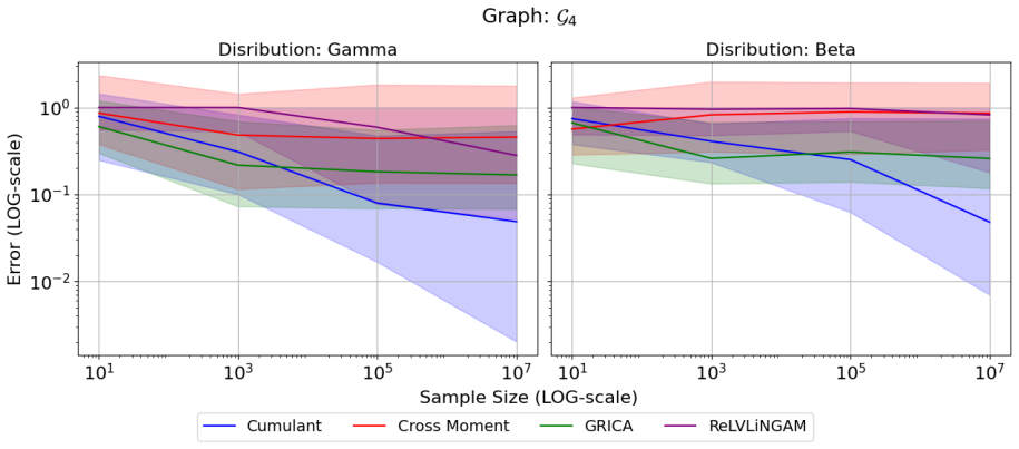
Figures from the paper (9 more)




Forward citations
Cited by 1 Pith paper
-
Latent Confounded Causal Discovery via Lie Bracket Geometry
Non-closing Lie brackets of intervention-response fields can serve as a high-recall screen for causal edges under latent confounding, but do not by themselves identify general DAGs.
Reference graph
Works this paper leans on
-
[1]
Let us call this polynomial map ψ and assume ψ(A) =ψ( ˜A)
It is clear that RG is the image of polynomial map ofRG A. Let us call this polynomial map ψ and assume ψ(A) =ψ( ˜A). Then from the definition of ψ we have (I−A o,o)−1 = (I− ˜Ao,o)−1 that implies Ao,o = ˜Ao,o. Moreover, (I−A o,o)−1Ao,l = (I− ˜Ao,o)−1 ˜Ao,l that impliesA o,l = ˜Ao,l and soA= ˜A. The isomorphisms between the rings come from Cox et al. (2015...
work page 2015
-
[3]
INPUT:DataV n = [Zn, Tn, Yn]. 1: ˆbY,T ←Algorithm3(V n) 2:b n Y,T ←arg min b∈R hVn,ˆbY T (b){(21)} 3:RETURN:b n Y,T In practice, we solve the optimization problem using the Python implementation of the BFGS algorithm (Nocedal & Wright, 2006, §6.1) provided in Jones et al. (2001–). The finite-sample version of this optimization process is detailed in Algorithm
work page 2006
-
[4]
RemarkC.1.If c(3)(L1)1,1,1 is zero, higher-order cumulants can be used to construct g(b). The existence of such a polynomial is guaranteed as long asL 1 is non-Gaussian; see, for example, Kivva et al. (2023, Thm. 1). C.2. Underspecified Instrumental Variable Algorithm 5 outlines the estimation procedure for causal effect estimation corresponding to the gr...
work page 2023
-
[7]
11 Causal Effect Identification in lvLiNGAM from Higher-Order Cumulants A. Notions of Non-Linear Algebra In this section, we give the basic definitions ofnon-linearalgebra we will need for the proofs; we refer the interested reader to Garcia et al. (2010); Cox et al. (2015); Michałek & Sturmfels (2021) for more details. Definition A.1.For every natural nu...
work page 2010
-
[8]
INPUT:Data Vn = [I n, T1 n . . . , Tk n , Yn, X1, . . . , Xe], the causal graph G, bound on the number of latent variables l. 1:Σ n ←c (2)(Vn){Sample covariance matrix} 2:ad(I, Y)←an(I)∩an(Y)∩ O {Valid adjustment set} 3:b Y,I,n ←(Σ n)Y,I|ad(I,Y) /(Σn)I,I|ad(I,Y) {Regression adjustment (Henckel et al., 2022, Prop. 1)} 4:Y I n ←Y n −b Y,I,n In {(17)} 5:for ...
work page 2022
-
[9]
, Tk, and outcome Y , and let l:= max i∈[n] |an(T i)∩an(Y)\I|
Theorem.Let GIV be an instrumental variable graph, with instrument I, treatments T 1, . . . , Tk, and outcome Y , and let l:= max i∈[n] |an(T i)∩an(Y)\I|. Then, the causal effect from T i to Y is generically identifiable from the first k(l) cumulants of the distribution. Proof of Theorem 3.7. Since an(I)∩an(T i)∩ L= an(I)∩an(Y)∩ L=∅ , we can identify bT i...
work page 2016
-
[13]
INPUT:DataV n = [I1 n, . . . , Is n, T1 n . . . , Tk n , Yn, X1, . . . , Xe], the causal graphG, bound on the number of latent variablesl. 1:Σ n ←c (2)(Vn){Sample covariance matrix} 2:for allj∈[s]do 3:ad(I j, Y)←an(I j)∩an(Y)∩ O {Valid adjustment set} 4:b Y,I j ,n ←(Σ n)Y,I j |ad(I j ,Y) /(Σn)I,I j |ad(I j ,Y) {Regression adjustment (Henckel et al., 2022,...
work page 2022
-
[2004]
Identifying causal effects with computer algebra
Garcia, L., Spielvogel, S., and Sullivant, S. Identifying causal effects with computer algebra. InUAI 2010, Pro- ceedings of the Twenty-Sixth Conference on Uncertainty in Artificial Intelligence, Catalina Island, CA, USA,
work page 2010
Show all 13 references
-
[2006]
Iden- tification and estimation of causal effects using non- gaussianity and auxiliary covariates.arXiv:2304.14895,
Shuai, K., Luo, S., Zhang, Y ., Xie, F., and He, Y . Iden- tification and estimation of causal effects using non- gaussianity and auxiliary covariates.arXiv:2304.14895,
-
[2008]
Jones, E., Oliphant, T., Peterson, P., et al
Special Section on Probabilistic Rough Sets and Special Section on PGM’06. Jones, E., Oliphant, T., Peterson, P., et al. SciPy: Open source scientific tools for Python, 2001–. URL http: //www.scipy.org/. Kilbertus, N., Rojas Carulla, M., Parascandolo, G., Hardt, M., Janzing, D...
2001
-
[2022]
Causal discovery of linear non-gaussian causal models with unobserved confounding.arXiv:2408.04907,
Schkoda, D., Robeva, E., and Drton, M. Causal discovery of linear non-gaussian causal models with unobserved confounding.arXiv:2408.04907,
-
[2023]
S., Kolar, M., and Drton, M
Wang, Y . S., Kolar, M., and Drton, M. Confidence sets for causal orderings.arXiv:2305.14506,
-
[2024]
Parameter identification in linear non-gaussian causal models under general confounding.arXiv:2405.20856, 2024a
Tramontano, D., Drton, M., and Etesami, J. Parameter identification in linear non-gaussian causal models under general confounding.arXiv:2405.20856, 2024a. Tramontano, D., Kivva, Y ., Salehkaleybar, S., Drton, M., and Kiyavash, N. Causal effect identification in lingam models ...
2024
Reviewed August 7, 2026 · model on record in the stance chip above.
Discussion (0). Sign in to comment.