REVIEW 5 minor 38 references
Approximate explicit formulas for Stoner-Wohlfarth hysteresis loops
T0 review · 0 major / 5 minor · reviewed 2026-07-14 · grok-4.5
Pith's one-line read Approximate elementary formulas reproduce Stoner–Wohlfarth hysteresis loops for single particles and random ensembles across the full field range.
desk verdict Clean, usable elementary approximations to SW loops that actually work; soft spots are openly quantified and do not sink the claim. read the letter →
The pith
A machine-rendered reading of the paper's core claim, the machinery that carries it, and where it could break.
The reading
What carries the argument
The low-field expansions for the equilibrium angle θ* (Eqs. 8–9) and the high-field expansion (Eq. 12), joined at hand-chosen matching fields (h0 = ±1.5 for fixed-angle loops, h0 = ±0.75 for the averaged loop) that minimize global deviation from the numerical solution.
What would settle it
Direct numerical comparison of the piecewise formulas against the exact energy-minimization solution of the Stoner–Wohlfarth equations over a dense grid of field values and easy-axis angles; if the absolute magnetization error systematically exceeds ~0.05 outside the immediate vicinity of switching, or if the averaged-loop coercivity error grows beyond a few percent, the claim fails.
Extended reading notes
Core claim
Piecewise elementary formulas, obtained by matching low-field (moment near easy axis) and high-field (moment near applied field) expansions at optimized intermediate points, reproduce the full Stoner–Wohlfarth hysteresis loops for both fixed easy-axis orientation and randomly oriented ensembles, with absolute magnetization error remaining below roughly 0.05 except near the switching field.
Load-bearing premise
The small-angle expansions that keep the magnetic moment near the easy axis remain accurate enough even near the Stoner–Wohlfarth switching curve, where the reduced field is no longer small.
Editorial extensions
If this is right
- Hysteresis loops for fixed-angle and randomly oriented SW particles can be evaluated with only elementary functions, without root-finding or angular integration.
- Initial susceptibilities of both single particles and random ensembles recover the known analytic limits of the model.
- The same piecewise construction supplies an explicit initial-magnetization curve for the random ensemble.
- The formulas remain usable near the switching field, where previous low-field approximations break down.
Reading between the lines
- The matching-field choice could be automated by a simple least-squares or minimax criterion, turning the present hand-tuned intervals into a fully algorithmic construction.
- Because the formulas are elementary, they can be embedded directly in larger micromagnetic or finite-element codes that currently call numerical SW solvers at every mesh point.
- The same low-/high-field matching strategy may extend to other uniaxial anisotropy models whose energy landscapes share a similar two-regime structure.
Signed reviews
Editorial analysis
A structured set of objections, weighed in public.
Referee Report
Summary. The paper derives approximate explicit piecewise formulas for Stoner–Wohlfarth hysteresis loops, both for a single particle at fixed easy-axis angle θ_H (Eqs. 16–20) and for an ensemble with randomly oriented anisotropy axes (Eqs. 50–55). The derivations rest on low-field small-angle expansions of the equilibrium condition (moment near the easy axis, Eqs. 8–9) and a high-field expansion (moment near the field direction, Eq. 12), with matching abscissae chosen to minimize global error against numerical solutions of the same model. Absolute deviations remain ≲0.05 over most of the field range, with the largest (still described as reasonably small) deviation near h_0≈0.5 for the averaged loop.
Significance. If the stated accuracy holds, the formulas supply a practical, elementary-function alternative to numerical root-finding and angular integration for the classic SW model. They rest on a transparent physical picture rather than pure least-squares parametrization, recover known limits (initial susceptibilities, approach-to-saturation law), and cover both fixed-orientation and random-ensemble cases. The internal validation against exact numerical solutions of the SW equations, together with the explicit inverse-astroid formulas in Appendix A, makes the results immediately usable for modeling nanoparticles, thin films, and polycrystalline magnets without statistical sampling.
minor comments (5)
- In §3.1–3.2 the small-angle approximations are introduced without an a-priori error bound; a short remark quantifying the maximum |θ′| or |θ*| on the astroid (already plotted in Fig. 5) would help the reader judge the domain of validity before the numerical checks of §6.
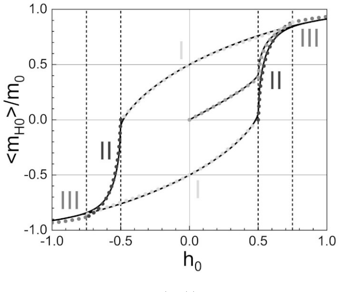
- The matching fields |h_0|=1.5 (fixed-θ_H) and |h_0|=0.75 (ensemble) are stated to be chosen for best fit, yet no sensitivity analysis is given. A single sentence or inset showing how the max |δ| changes if the join is moved by ±0.1 would strengthen the claim that the choice is robust.
- Figure 2 caption and the surrounding text refer to “dotted curves” for the analytic formulas, but the line styles are hard to distinguish in grayscale; adding a legend or using dashed/solid consistently would improve readability.
- Eq. (23) for the initial curve at fixed θ_H is left in a rather cumbersome product-of-sines form; a brief expansion for small h_0 would make the connection to the known χ_max = M_0²/(2K_a) more transparent.
- Typographical: in the abstract and highlights the arXiv identifier appears as 2607.09881 while the header uses the same; consistency with the final journal citation style should be checked at proof stage.
Circularity Check
No significant circularity: approximations are asymptotic expansions of the SW equilibrium equation, assembled piecewise and validated against independent numerical solutions of the same model.
full rationale
The derivation chain begins from the exact SW reduced energy (Eq. 1) and equilibrium condition (Eq. 3). Low-field (sin heta'≈ heta', cos heta'≈1) and high-field expansions then produce the explicit heta* approximations (Eqs. 8, 9, 12) that are substituted into the projection m_H0/m0=cos( heta*- heta_H) and, for the ensemble, into the orientation integral (Eq. 24). The resulting piecewise elementary expressions (fixed- heta_H: Eqs. 16–20; random: Eqs. 50–55) are therefore approximate solutions of the model itself. Matching abscissae (h0=±1.5, ±0.75) and the order of the logarithm expansion are chosen post-hoc to minimize absolute deviation from numerical solutions of the identical SW equations; this is ordinary engineering of an approximation, not a fit of free parameters that are later re-labeled as independent predictions. No self-citation supplies a load-bearing uniqueness claim, no ansatz is smuggled via prior work of the authors, and the formulas are not definitional rearrangements of their inputs. The paper is self-contained against its own numerical benchmarks; circularity score is therefore zero.
Assumptions & free parameters
free parameters (3)
- matching field |h0|=1.5 (fixed-angle loops)
- matching fields |h0|=0.75 and 0.5 (ensemble loops)
- third-order truncation of ln(1-h0)
assumptions (3)
- domain assumption Stoner–Wohlfarth reduced energy w = (1/2)sin^{2}θ − h0 cos(θ−θH) and the associated equilibrium/stability conditions (Eqs. 1–4)
- ad hoc to paper Small-angle approximations sin θ′≈θ′, cos θ′≈1 (and likewise for θ″) when the moment is near the easy axis or the field direction
- domain assumption Uniform (isotropic) distribution of anisotropy axes for the ensemble average (Eq. 24)
Cite this review
Pith. "Pith review of Approximate explicit formulas for Stoner-Wohlfarth hysteresis loops." pith.science (2026). https://pith.science/paper/LGYFFXMD
@misc{pith2026260709881,
  author       = {Pith},
  title        = {Pith review of: Approximate explicit formulas for Stoner-Wohlfarth hysteresis loops},
  year         = {2026},
  howpublished = {\url{https://pith.science/paper/LGYFFXMD}},
  note         = {Machine review of arXiv:2607.09881}
}
read the original abstract
Approximate explicit formulas for the hysteresis loops in the Stoner-Wohlfarth model are derived. We consider the hysteresis loops both for a single particle with a fixed easy-axis direction and for an ensemble of particles with randomly oriented anisotropy axes. The physical assumption used to derive the formulas is that the particle magnetic moment lies in the vicinity of the easy axis or the external field direction, at low and high fields, respectively. Surprisingly, the low-field formula is approximately valid even near the Stoner-Wohlfarth astroid, where the reduced magnetic field h0 is not very small. The general piecewise formula is obtained by an appropriate matching of the functions defined on different intervals of the magnetic field, which are chosen to maximize the formula accuracy. For the averaged hysteresis loop, the maximal, but reasonably small, deviation of our formula from numerically calculated magnetization occurs at h0 = 0.5, which corresponds to the sharp change in magnetization slope.
Figures


Figures from the paper (4 more)


Reference graph
Works this paper leans on
-
[1]
Bertotti, Hysteresis in magnetism: for physicists, materials scientists, and engineers, Academic press, 1998
G. Bertotti, Hysteresis in magnetism: for physicists, materials scientists, and engineers, Academic press, 1998
1998
-
[2]
A. H. Morrish, The Physical Principles of Magnetism, John Wiley and Sons, 2001
2001
-
[3]
D. Jiles, Hysteresis models: non-linear magnetism on length scales from the atomistic to the macroscopic, Journal of Magnetism and Magnetic Materi- als 242-245 (2002) 116–124, proceedings of the Joint European Magnetic Symposia (JEMS’01). doi:10.1016/S0304-8853(01)01213-6
-
[4]
D. C. Jiles, X. Fang, W. Zhang, Modeling of Hysteresis in Magnetic Mate- rials, Springer US, Boston, MA, 2006, pp. 745–779. doi:10.1007/1-4020- 7984-2_17
doi:10.1007/1-4020- 2006
-
[5]
M. Hodgdon, Mathematical theory and calculations of magnetic hystere- sis curves, IEEE Transactions on Magnetics 24 (6) (1988) 3120–3122. doi:10.1109/20.92354
-
[6]
D. Atherton, J. Beattie, A mean fieldStoner–Wohlfarthhysteresis model, IEEE Transactions on Magnetics 26 (6) (1990) 3059–3063. doi:10.1109/20.102891
-
[7]
H. Hauser, Energetic model of ferromagnetic hysteresis, Journal of Applied Physics 75 (5) (1994) 2584–2597. doi:10.1063/1.356233
-
[8]
Della Torre, et al., Magnetic hysteresis, IEEE press, 1999
E. Della Torre, et al., Magnetic hysteresis, IEEE press, 1999
1999
Show all 38 references
-
[9]
E. Della Torre, Problems in physical modeling of magnetic materials, Physica B: Condensed Matter 343 (1) (2004) 1–9, proceedings of the Fourth Intional Conference on Hysteresis and Micromagnetic Modeling. doi:10.1016/j.physb.2003.08.052
2004 doi
-
[10]
N. C. Pop, A model for magnetic hysteresis, The European Physical Journal Plus 134 (11) (2019) 567
2019
-
[11]
Mörée, M
G. Mörée, M. Leijon, Review of hysteresis models for magnetic materials, Energies 16 (9) (2023). doi:10.3390/en16093908. 33
2023 doi
-
[12]
I. D. Mayergoyz, Mathematical models of hysteresis and their applications, Academic press, 2003
2003
-
[13]
Liorzou, B
F. Liorzou, B. Phelps, D. Atherton, Macroscopic models of mag- netization, IEEE Transactions on Magnetics 36 (2) (2000) 418–428. doi:10.1109/20.825802
2000 doi
-
[14]
E. C. Stoner, E. P. Wohlfarth, A mechanism of magnetic hysteresis in hetero- geneous alloys, Philosophical Transactions of the Royal Society of London. Series A, Mathematical and Physical Sciences 240 (826) (1948) 599–642. doi:10.1098/rsta.1948.0007
1948 doi
-
[15]
Tannous, J
C. Tannous, J. Gieraltowski, TheStoner–Wohlfarthmodel of ferromag- netism, European Journal of Physics 29 (3) (2008) 475. doi:10.1088/0143- 0807/29/3/008
2008 doi
-
[16]
M. A. Chuev, J. Hesse, Nanomagnetism: extension of theStoner–Wohlfarth model withinNéel’s ideas and useful plots, Journal of Physics: Condensed Matter 19 (50) (2007) 506201
2007
-
[17]
Tamion, E
A. Tamion, E. Bonet, F. Tournus, C. Raufast, A. Hillion, O. Gaier, V . Dupuis, Efficient hysteresis loop simulations of nanoparticle assem- blies beyond the uniaxial anisotropy, Phys. Rev. B 85 (2012) 134430. doi:10.1103/PhysRevB.85.134430
2012 doi
-
[18]
Jubert, Micromagnetic simulations of exchange-coupled core–shell particulate media, IEEE Transactions on Magnetics 50 (11) (2014) 1–4
P.-O. Jubert, Micromagnetic simulations of exchange-coupled core–shell particulate media, IEEE Transactions on Magnetics 50 (11) (2014) 1–4. doi:10.1109/TMAG.2014.2327613
2014 doi
-
[19]
Coïsson, G
M. Coïsson, G. Barrera, C. Appino, F. Celegato, L. Martino, A. P. Safronov, G. V . Kurlyandskaya, P. Tiberto, Specific loss power measurements by calorimetric and thermal methods onγ-Fe 2O3 nanoparticles for magnetic hyperthermia, Journal of Magnetism and Magnetic Materials 47...
2019 doi
-
[20]
S. V . Komogortsev, D. A. Balaev, A. A. Krasikov, S. V . Stolyar, R. N. Yaroslavtsev, V . P. Ladygina, R. S. Iskhakov, Magnetic hysteresis of blocked ferrihydrite nanoparticles, AIP Advances 11 (1) (2021) 015329. doi:10.1063/9.0000111. 34
2021 doi
-
[21]
Anand, Hysteresis in a linear chain of magnetic nanoparticles, Journal of Applied Physics 128 (2) (2020) 023903
M. Anand, Hysteresis in a linear chain of magnetic nanoparticles, Journal of Applied Physics 128 (2) (2020) 023903. doi:10.1063/5.0010217
2020 doi
-
[22]
Delgado-Garcia, G
R. Delgado-Garcia, G. Rodriguez-Rodriguez, J. M. Colino, Improved averaging of hysteresis loops from micromagnetic simulations of non- interacting uniaxial nanoparticles, AIP Advances 11 (1) (2021) 015137. doi:10.1063/9.0000158
2021 doi
-
[23]
Mörée, J
G. Mörée, J. Sjölund, M. Leijon, A review of permanent magnet models used for designing electrical machines, IEEE Transactions on Magnetics 58 (11) (2022) 1–19. doi:10.1109/TMAG.2022.3200150
2022 doi
-
[24]
K. R. Coffey, T. Thomson, J.-U. Thiele, Angle dependent magnetization re- versal of thin film magnetic recording media, Journal of Applied Physics 93 (10) (2003) 8471–8473. doi:10.1063/1.1540167
2003 doi
-
[25]
J. C. Slonczewski, Theory of magnetic hysteresis in films and its applica- tion to computers, IEEE Transactions on Magnetics 45 (1) (2009) 8–14. doi:10.1109/TMAG.2008.2008671
2009 doi
-
[26]
T. M. L. Alves, C. G. Bezerra, A. D. C. Viegas, S. Nicolodi, M. A. Cor- rêa, F. Bohn, Quantifying magnetic anisotropy dispersion: Theoretical and experimental study of the magnetic properties of anisotropicFeCuNbSiB ferromagnetic films, Journal of Applied Physics 117 (8) (2015...
2015 doi
-
[27]
J. L. F. Cuñado, A. Bollero, T. Pérez-Castañeda, P. Perna, F. Ajejas, J. Pe- drosa, A. Gudín, A. Maldonado, M. A. Niño, R. Guerrero, et al., Emergence of theStoner–Wohlfarthastroid in thin films at dynamic regime, Scientific reports 7 (1) (2017) 13474
2017
-
[28]
Ikegawa, F
S. Ikegawa, F. B. Mancoff, J. Janesky, S. Aggarwal, Magnetoresistive ran- dom access memory: Present and future, IEEE Transactions on Electron Devices 67 (4) (2020) 1407–1419. doi:10.1109/TED.2020.2965403
2020 doi
-
[29]
P. D. Dimitropoulos, G. I. Stamoulis, E. Hristoforou, A 3-DhybridJiles- Atherton/Stoner-Wohlfarthmagnetic hysteresis model for inductive sen- sors and actuators, IEEE Sensors Journal 6 (3) (2006) 721–736. 35
2006
-
[30]
Wood, Exact solution for aStoner–Wohlfarthparticle in an applied field and a new approximation for the energy barrier, IEEE Transactions on Mag- netics 45 (1) (2009) 100–103
R. Wood, Exact solution for aStoner–Wohlfarthparticle in an applied field and a new approximation for the energy barrier, IEEE Transactions on Mag- netics 45 (1) (2009) 100–103. doi:10.1109/TMAG.2008.2006286
2009 doi
-
[31]
N. A. Zarkevich, C. I. Nlebedim, R. W. McCallum, Parame- terization of theStoner–Wohlfarthmodel of magnetic hysteresis, Journal of Magnetism and Magnetic Materials 530 (2021) 167913. doi:https://doi.org/10.1016/j.jmmm.2021.167913
2021 doi
-
[32]
C. A. Iglesias, J. C. R. de Araújo, E. F. Silva, M. Gamino, M. A. Correa, F. Bohn, Fundamental inequalities in theStoner–Wohlfarthmodel, Phys. Rev. B 106 (2022) 094405. doi:10.1103/PhysRevB.106.094405
2022 doi
-
[33]
Appino, Exact formulation for hysteresis loops and energy loss inStoner–Wohlfarthsystems, AIP Advances 13 (5) (2023) 055018
C. Appino, Exact formulation for hysteresis loops and energy loss inStoner–Wohlfarthsystems, AIP Advances 13 (5) (2023) 055018. doi:10.1063/5.0143905
2023 doi
-
[34]
J. M. Coey, Magnetism and magnetic materials, Cambridge university press, 2010
2010
-
[35]
O’Grady, R
K. O’Grady, R. Chantrell, J. Popplewell, S. Charles, The low temperature magnetisation of a system of fine cobalt particles, IEEE Transactions on Magnetics 16 (5) (1980) 1077–1079. doi:10.1109/TMAG.1980.1060827
1980 doi
-
[36]
Akulov, Über die anwendungen des gesetzes ferromagnetischer anisotropie zur berechnung der eigenschaften polykristallinischen eisens, Zeitschrift für Physik 66 (7) (1930) 533–542
N. Akulov, Über die anwendungen des gesetzes ferromagnetischer anisotropie zur berechnung der eigenschaften polykristallinischen eisens, Zeitschrift für Physik 66 (7) (1930) 533–542
1930
-
[37]
Holstein, H
T. Holstein, H. Primakoff, Magnetization near saturation in polycrystalline ferromagnets, Phys. Rev. 59 (1941) 388–394. doi:10.1103/PhysRev.59.388
1941 doi
-
[38]
E. C. Devi, S. D. Singh, Tracing the magnetization curves: a review on their importance, strategy, and outcomes, Journal of Superconductivity and Novel Magnetism 34 (1) (2021) 15–25. 36
2021
Reviewed July 14, 2026 · model on record in the stance chip above.
Discussion (0). Continue with ORCID to comment.