REVIEW 2 major objections 7 minor 121 references
Provable bounds for the Korteweg-de Vries reduction in multi-component Nonlinear Schrodinger Equation
T0 review · 2 major / 7 minor · reviewed 2026-08-14 · deepseek-v4-flash
Pith's one-line read This paper aims to prove that small perturbations of an N-component Nonlinear Schrödinger (Gross–Pitaevskii) system are governed, at long times, by Korteweg–de Vries equations, one per sound-speed mode, with coefficients fixed by the…
desk verdict Solid formal KdV reduction with a rigorous spectral core, but the numerical validation uses a soliton that is not a solution of the derived KdV equation, and the title's 'provable bounds' are not delivered. read the letter →
The pith
A machine-rendered reading of the paper's core claim, the machinery that carries it, and where it could break.
The reading
What carries the argument
The load-bearing object is the $2N \times 2N$ matrix $A$ whose block form is $\begin{pmatrix}0&\rho\\\alpha&0\end{pmatrix}$, obtained from the linearized hydrodynamic equations. Its eigenvalues are the sound speeds, and its eigenvectors determine the KdV coefficients. The argument proceeds through a sequence of theorems: eigenvalues of $A$ are real and paired when $\alpha$ is positive definite; permanent degeneracy occurs exactly when pairs $(\rho_{0i}g_i,\rho_{0i})$ coincide; and $A$ is diagonalizable. A reductive multiple-scales perturbation, with the Fredholm alternative enforcing solvability of the linearized inhomogeneous equation, converts the first nonlinear correction into the KdV system. The eigenvector matrix $V$ and its inverse transpose are expressed in terms of the eigenvectors of $\rho\alpha$, reducing the whole computation to the spectrum of that matrix.
What would settle it
Evolve a three-component NLS with three well-separated sound speeds and compare each moving frame's density profile to the predicted KdV equations: if the envelope speed or shape deviates by more than the expected $O(\epsilon^3)$ error, the asymptotic reduction fails. Alternatively, tune two sound speeds close together and check whether the two KdV channels remain independent; energy exchange between channels at small $\epsilon$ would contradict the uncoupling premise.
Extended reading notes
Core claim
The central claim is that for an $N$-component system with symmetric positive-definite coupling matrix $\alpha$ and positive background densities, small perturbations separate into $2N$ weakly nonlinear waves, one for each sound speed, and each wave envelope satisfies a KdV equation. After the standard scaling $x,t \mapsto \epsilon x,\epsilon t$ and amplitude $\epsilon^2$, the derivation yields for each eigenvalue $\lambda_j$ of $A$ an equation of the form $\partial_\tau f_j + B_j f_j f_{j\xi} + A_j f_{j\xi\xi\xi}=0$, with $A_j,B_j$ computed from the eigenvectors. For distinct eigenvalues the equations are uncoupled. The paper obtains this through a Fredholm-alternative solvability condition at the first nonlinear order, gives explicit coefficients for $N=2$ and $N=3$, and identifies a special case in which the nonlinear coefficient vanishes so the effective equation is linear.
Load-bearing premise
The derivation assumes the sound speeds—the eigenvalues of $A$—are distinct; when two coincide, the paper does not establish the claimed uncoupled KdV description and explicitly leaves that case to future work.
Editorial extensions
If this is right
- For any $N$ with distinct sound speeds, a generic small perturbation resolves into $2N$ independent KdV waves; measuring the wave speeds determines products of background densities and couplings.
- The reduction places dispersion and nonlinearity on the same footing, so KdV solitons can be used to prepare and predict coherent density dips and bumps in multi-component condensates.
- The explicit $N=2$ coefficients allow quantitative lab-frame predictions of soliton speeds, including the reversal from a density bump to a density dip between species.
- In the special case of equal self-couplings and equal background densities, the effective KdV equation is linear, so that mode does not form solitons.
- The iterative spectral algorithm tracks how sound speeds and KdV coefficients change with the tunable cross-coupling $h$, which is directly relevant to Feshbach-resonance experiments.
Reading between the lines
- For repeated sound speeds, the same machinery likely yields a coupled system of KdV equations whose coefficients come from the degenerate eigenvectors provided by Theorem 6; the paper leaves this case explicitly open.
- When two sound speeds are nearly equal but not exactly equal, the formal uncoupled description may fail on observable timescales; an experiment scanning $h$ through an avoided crossing could expose emergent coupling not visible in the $\epsilon$-expansion.
- Because the reduction uses only local hydrodynamic structure, analogous KdV descriptions should hold for other multi-component NLS-type settings such as optical pulses and plasma waves, not only cold atoms.
- The method may extend to spatially varying couplings or external potentials by promoting the constants to slowly varying coefficients, though the paper notes that this remains unexplored.
Signed reviews
Editorial analysis
A structured set of objections, weighed in public.
Referee Report
Summary. The paper studies the multi-component nonlinear Schrödinger equation (VNLS/VGPE) in one spatial dimension. After a Madelung transformation, the authors linearize about a constant background and provide a rigorous spectral analysis of the 2N×2N operator A that governs the linearized hydrodynamic equations. Under the special form of the coupling matrix αij = gi δij + h(1−δij), they characterize the characteristic polynomial, give conditions for repeated eigenvalues, and construct the associated eigenvectors. Using a formal multiple-scales expansion in a small parameter ε² and the Fredholm alternative, they derive 2N KdV equations for the amplitudes of the right- and left-moving waves, with coefficients determined by the eigenvectors of A. Explicit coefficients are given for N = 2 and N = 3, and a numerical comparison between the two-component NLS and the corresponding KdV equation is presented using a sech² solitary-wave profile.
Significance. If the derivation were made rigorous with error estimates, the paper would provide a systematic and explicit KdV reduction for an arbitrary number of components, together with a complete spectral characterization of the linearized problem. The spectral theorems (Theorems 1–6) are real mathematical statements with proofs in the appendices, and the KdV coefficients are derived from the linearized operator rather than fitted to NLS data, which is a genuine strength. However, the advertised 'provable bounds' are entirely absent, and the numerical validation is built on a solitary-wave profile that does not solve the derived KdV equation. The central formal reduction may be correct, but the evidence presented for it is currently not sound.
major comments (2)
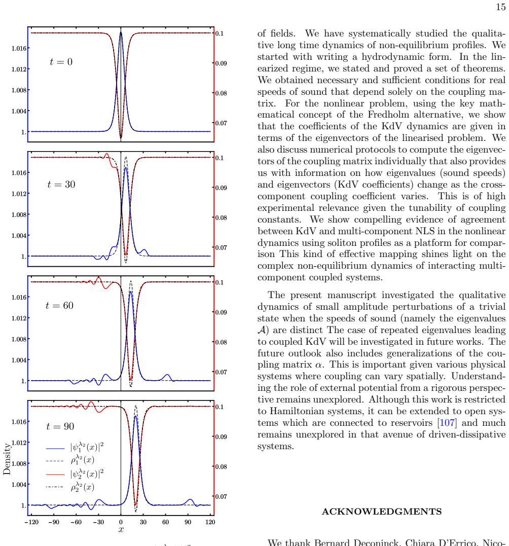
- [Section V, Eq. (100)] The function f_j(ξ,τ) = (3 V A_j/B_j) sech²(√(V/2)(ξ − A_j V τ)) is not a solution of the KdV equation (80), ∂τ f + B_j f f′ + A_j f‴ = 0. For a soliton of the form a sech²(k(ξ − cτ)), substitution into (80) requires a = 12 A_j k²/B_j and c = 4 A_j k². With k² = V/2, Eq. (100) gives a = 3 V A_j/B_j and c = A_j V, which differ from the required values by a factor of two in both amplitude and speed. Consequently, the initial conditions (103)–(104), the lab-frame speed Λ_j = λ_j + A_j V ε² in Eq. (105), and the analytical density curves in Figs. 1–2 are not the KdV soliton of the equation being tested. The numerical comparison therefore cannot confirm the KdV reduction as claimed; the soliton formula (or the KdV normalization) must be corrected and the simulations rerun.
- [Title, Abstract, and Section III] The paper advertises 'Provable bounds for the Korteweg–de Vries reduction', but the manuscript contains no bound on the difference between solutions of the original VNLS and solutions of the reduced KdV equation. The derivation in Section III is a formal multiple-scales expansion; no remainder estimate, convergence statement, or validity time-scale is supplied. The rigorous component is the spectral analysis of the linear operator A, not the nonlinear reduction. The title and abstract should be revised to describe a formal asymptotic reduction accompanied by rigorous spectral analysis, or the authors should supply actual error bounds; otherwise the advertised central contribution is not delivered.
minor comments (7)
- [Theorems 4 and 6] The multiplicity conventions in Theorems 4 and 6 are inconsistent: Theorem 4 states that m equal pairs produce an eigenvalue of multiplicity m−1, while Theorem 6 assumes an eigenvalue of multiplicity m and constructs m eigenvectors from m+1 equal pairs. The text should be harmonized so that the reader can compare the two statements without confusion.
- [Introduction and Section II.3] The introduction states that the paper gives necessary and sufficient conditions for sound speeds to be distinct; what is actually proved in Theorem 4 is a condition for permanent degeneracy of the characteristic polynomial. Since isolated collisions of eigenvalues can occur for particular values of h even when the permanent-degeneracy condition fails, the wording should be adjusted to match the theorem.
- [Abstract and title] The title and abstract use 'Korteweg de-Vries' and 'provable bounds'; the former should be 'Korteweg–de Vries' and the latter is misleading (see Major Comment 2).
- [Figure captions] In Figure 2 the caption contains 'secondand largest', which should read 'second largest'; in Figure 1 the caption reads 'are evolve', which should be 'evolve'.
- [Equation (106c)] Equation (106c) contains a typo in the parentheses: 'ρλ2 1 x,t ) =' should be 'ρλ2_1(x,t) ='.
- [Equation (105)] Equation (105) refers to Λ_j as the speed of sound in the lab frame; Λ_j is the solitary-wave speed, not the linear sound speed. This terminology should be clarified.
- [Reference [42]] Reference [42] is incomplete: it lists only a journal volume and no authors or title.
Circularity Check
No circularity: the KdV coefficients are computed from the linearized eigenproblem and no fitted parameter is renamed as a prediction; the main limitations and the flawed numerical soliton formula are correctness issues, not circular inputs.
full rationale
The derivation chain is self-contained. The KdV reduction in Section III starts from the hydrodynamic form (40)-(42) that is equivalent to the original VNLS via the Madelung transform, expands solutions as (47), and obtains the solvability condition (55)-(56) by projecting the O(epsilon^2) nonlinear terms onto the adjoint nullspace. The KdV coefficients A_j and B_j in the N=2 and N=3 cases, eqs. (80)-(84) and (91)-(97), are explicit algebraic functions of the coupling matrix alpha, the background densities rho0, and the eigenvectors of the linearized operator A; none of these coefficients is fitted to NLS data or to the numerical comparison. The numerical test in Section V uses independent initial data built from the KdV solitary-wave formula (100) and compares the subsequent NLS evolution with the corresponding analytical densities, so it is not a fit by construction. The manuscript is also explicit about its scope: Section II.3 states 'If the conditions for case (b) are not satisfied, then we will assume the eigenvalues are simple for a given h,' and Section VI states 'The case of repeated eigenvalues leading to coupled KdV will be investigated in future works.' That is a stated limitation rather than a circular assumption. The paper cites prior work by its own authors (e.g. Ref. [24] and an unpublished Ref. [107]), but these citations are contextual or programmatic and are not load-bearing in the derivation; no uniqueness theorem or ansatz is imported from those citations. One non-circular correctness concern should be flagged: Eq. (100) does not solve the KdV equation (80) as written; for f = alpha sech^2(k(xi-c tau)) the KdV coefficients require alpha = 12 A_j k^2 / B_j and c = 4 A_j k^2, while (100) gives alpha = 3 V A_j / B_j and c = A_j V with k = sqrt(V/2). This invalidates the numerical benchmark in Section V, but it is an internal error in the validation, not a reduction of the claimed KdV law to its inputs. The central asymptotic derivation remains independent of the numerical comparison.
Assumptions & free parameters
assumptions (5)
- domain assumption The coupling matrix α is real, symmetric, positive definite, with diagonal g_i and off-diagonal h (Assumption 1).
- domain assumption The background densities ρ0k are positive.
- ad hoc to paper The formal perturbation expansion in ε² is asymptotically valid.
- domain assumption The eigenvalues of A (sound speeds) are simple for the h considered.
- standard math Standard Fredholm alternative and implicit function theorem for finite-dimensional matrices.
Cite this review
Pith. "Pith review of Provable bounds for the Korteweg-de Vries reduction in multi-component Nonlinear Schrodinger Equation." pith.science (2026). https://pith.science/paper/LH4DVZT3
@misc{pith2026190802248,
  author       = {Pith},
  title        = {Pith review of: Provable bounds for the Korteweg-de Vries reduction in multi-component Nonlinear Schrodinger Equation},
  year         = {2026},
  howpublished = {\url{https://pith.science/paper/LH4DVZT3}},
  note         = {Machine review of arXiv:1908.02248}
}
read the original abstract
We study the dynamics of multi-component Bose gas described by the Vector Nonlinear Schr\"{o}dinger Equation (VNLS), aka the Vector Gross--Pitaevskii Equation (VGPE) . Through a Madelung transformation, the VNLS can be reduced to coupled hydrodynamic equations in terms of multiple density and velocity fields. Using a multi-scaling and a perturbation method along with the Fredholm alternative, we reduce the problem to a Korteweg de-Vries (KdV) system. This is of great importance to study more transparently, the obscure features hidden in VNLS. This ensures that hydrodynamic effects such as dispersion and nonlinearity are captured at an equal footing. Importantly, before studying the KdV connection, we provide a rigorous analysis of the linear problem. We write down a set of theorems along with proofs and associated corollaries that shine light on the conditions of existence and nature of eigenvalues and eigenvectors of the linear problem. This rigorous analysis is paramount for understanding the nonlinear problem and the KdV connection. We provide strong evidence of agreement between VNLS systems and KdV equations by using soliton solutions as a platform for comparison. Our results are expected to be relevant not only for cold atomic gases, but also for nonlinear optics and other branches where VNLS equations play a defining role.
Figures

Reference graph
Works this paper leans on
-
[1]
This regime naturally leads to a coupled multi-species KdV- like model
Modeling As mentioned in the introduction, one of the pri- mary contributions of the present manuscript is a char- acterization of a multicomponent system, particularly in the small-amplitude long-wavelength regime. This regime naturally leads to a coupled multi-species KdV- like model. In order to derive the associated KdV model, we first perform the usua...
-
[2]
A natural question is how small perturbations to this background state evolve
Linearized dynamics A trivial solution to the hydrodynamic equations is given by setting the densities to non-negative constants ρ0k and the velocities to zero. A natural question is how small perturbations to this background state evolve. The standard approach to this question is given by linearising the equations about the background state, namely setti...
-
[3]
As we will see in the following section, both eigenvalues and eigenvectors play a key role in deriving equations governing the nonlinear dynamics of small am- plitude pulses
Spectral analysis of A As emphasized in the previous section, the eigenvalues ofA play a crucial role in designing the multicomponent system. As we will see in the following section, both eigenvalues and eigenvectors play a key role in deriving equations governing the nonlinear dynamics of small am- plitude pulses. The purpose of the present section is to...
-
[4]
represent the repeated pair resulting in the degenerate eigenvalue. A set of m independent eigenvectors for these permanently degenerate eigenval- ues λ =± √ ρ∗ 0(g∗ 0−h) of multiplicity m are given by v(k) = ±1√ ρ∗ 0(g∗ 0−h) ρq(k) q(k) , (25) where the i−th component of the k−th eigenvector is given by (q(k))i = 1, i =i1, −1, i =ik+1, 0, e...
-
[5]
The main tool we employ is the Fredholm alternative
Inhomogeneous linear dynamics With an eye towards the calculations in the next sec- tion, we now discuss the solution procedure for inhomo- geneous equations of the form (∂T +A∂X)s =f, A = ( 0 ρ α 0 ) (37) where we assumef is a knownN× 1 vector valued func- tion and we wish to determine the N× 1 vector s. The main tool we employ is the Fredholm alternativ...
-
[6]
This is however not the most general solution
Coupled KdV equations (non-distinct speeds) In the derivation presented in the previous section we assumed a solution to the homogeneous problem that de- pended only on one profile f (0) j . This is however not the most general solution. Indeed one may have well assumed V−1 ( δρ(0) δv (0) ) = ∑ j f (0) j (X−λjT,ϵ 2T )ej. (58) Evidently now ∂XV−1 ( N1(δρ(0)...
-
[7]
In other 10 words αρQ = QΛ2
Some useful relations Suppose Q is the matrix of eigenvectors of αρ with eigenvalues given by the diagonal matrix Λ 2. In other 10 words αρQ = QΛ2. All diagonal entries of Λ 2 are posi- tive (see proof of Theorem 5). Then the matrix of eigen- vectors forA is given by V = ( ρQΛ−1 −ρQΛ−1 Q Q ) , (61) with inverse V−1 = 1 2 ( ΛQ−1ρ−1 Q−1 −ΛQ−1ρ−1 Q−1 ) . (62...
-
[8]
Let us con- sider a case when two self-couplings (diagonal elements ofα) and their corresponding background states (the re- spective diagonal elements ofρ) are equal
A special case: KdV with zero nonlinearity The matrix α represents the coupling between the dif- ferent species and the matrix ρ represents the trivial background states for the different species. Let us con- sider a case when two self-couplings (diagonal elements ofα) and their corresponding background states (the re- spective diagonal elements ofρ) are e...
Show all 121 references
-
[9]
Remarkably this equation is linear and thus readily solved using Fourier transform techniques
Thus ˜v = √ ρ∗ 0 (g∗−h) 4ρ∗ 0 q 1 4q (71) 11 Then the KdV equation is given by fτ + ⟨ ˜v,∂X N1 ( ρ√ ρ∗ 0(g∗−h) q,q ) N2 ( ρ√ ρ∗ 0(g∗−h) q,q, 0 ) ⟩ = 0, (72) which upon simplifying is fτ− ℏ2 8 √ ρ∗ 0(g∗−h) f′′′ = 0, (73) wheref′′′ denotes the third-deriv...
-
[10]
(40) to (42) where k = 1, 2
N = 2 case The coupled NLS are as follows iℏ∂ψ1 ∂t =− ℏ2 2m ∂2ψ1 ∂x2 +g1|ψ1|2ψ1 +h|ψ2|2ψ1 (74a) iℏ∂ψ2 ∂t =− ℏ2 2m ∂2ψ2 ∂x2 +h|ψ1|2ψ2 +g2|ψ2|2ψ2 (74b) In other words, the α matrix (under the assumption m = 1; see text below Assumption 1) is given by α = ( g1 h h g 2 ) (75) The ...
-
[11]
N = 3 case The N = 3 case poses an interesting scenario. In gen- eral, for arbitraryg1,g 2,g 3 andρ01,ρ 02,ρ 03 (all different) the eigenvalues are very cumbersome but with our pre- scription outlined in the previous sections one can explic- itly write it down. Below, we descri...
2016
-
[12]
We consider first m repeated pairs of (ρ0igi,ρ 0i) and prove this is a sufficient condition to guarantee a repeated eigenvalue
Proof of sufficiency We now proceed to the general case. We consider first m repeated pairs of (ρ0igi,ρ 0i) and prove this is a sufficient condition to guarantee a repeated eigenvalue. Let (ρ∗ 0,g∗) denote the common value ofm repeated pairs of (ρ0i,gi). Since the total number of e...
-
[13]
To show this we prove the contrapositive, i.e
Proof of necessity It is also necessary that at least three pairs of (ρ0igi,ρ 0i) be equal for the characteristic polynomial to be permanently degenerate. To show this we prove the contrapositive, i.e. we show that if only m = 1, 2 of the (ρ0igi,ρ 0i) pairs are equal, then the...
-
[14]
Let the common value be (ρ∗ 0g∗,ρ∗ 0)
Suppose only two of the (ρ0igi,ρ 0i) are equal. Let the common value be (ρ∗ 0g∗,ρ∗ 0). By assumption this common value is distinct from all remainingN−2 (ρ0igi,ρ 0i) pairs. Factoring as we did previously, but for the case m = 2, we have Q(µ) = (ρ∗ 0g∗−µ ρ∗ 0h − 1 ) × [N−2∑ p=0...
-
[15]
Smerzi, A
A. Smerzi, A. Trombettoni, T. Lopez-Arias, C. Fort, P. Maddaloni, F. Minardi, and M. Inguscio, The Euro- pean Physical Journal B-Condensed Matter and Com- plex Systems 31, 457 (2003)
2003
-
[16]
Burchianti, C
A. Burchianti, C. D’Errico, S. Rosi, A. Simoni, M. Mod- ugno, C. Fort, and F. Minardi, Phys. Rev. A 98, 063616 (2018)
2018
-
[17]
Roati, M
G. Roati, M. Zaccanti, C. DErrico, J. Catani, M. Mod- ugno, A. Simoni, M. Inguscio, and G. Modugno, Phys- ical review letters 99, 010403 (2007)
2007
-
[18]
Thalhammer, G
G. Thalhammer, G. Barontini, L. De Sarlo, J. Catani, F. Minardi, and M. Inguscio, Physical review letters 100, 210402 (2008)
2008
-
[19]
Ejnisman, H
R. Ejnisman, H. Pu, Y. E. Young, N. P. Bigelow, and C. Law, Optics express 2, 330 (1998)
1998
-
[20]
Wacker, N
L. Wacker, N. B. Jørgensen, D. Birkmose, R. Horchani, W. Ertmer, C. Klempt, N. Winter, J. Sherson, and J. J. Arlt, Physical Review A 92, 053602 (2015)
2015
-
[21]
McCarron, H
D. McCarron, H. Cho, D. Jenkin, M. K¨ oppinger, and S. Cornish, Physical Review A 84, 011603 (2011)
2011
-
[22]
S. Papp, J. Pino, and C. Wieman, Physical review let- ters 101, 040402 (2008)
2008
-
[23]
F. Wang, X. Li, D. Xiong, and D. Wang, Journal of Physics B: Atomic, Molecular and Optical Physics 49, 015302 (2015)
2015
-
[24]
Matthews, B
M. Matthews, B. P. Anderson, P. Haljan, D. Hall, M. Holland, J. Williams, C. Wieman, and E. Cornell, Physical review letters 83, 3358 (1999)
1999
-
[25]
Z. Chen, M. Segev, T. H. Coskun, D. N. Christodoulides, and Y. S. Kivshar, JOSA B 14, 20 3066 (1997)
1997
-
[26]
E. A. Ostrovskaya, Y. S. Kivshar, Z. Chen, and M. Segev, Optics letters 24, 327 (1999)
1999
-
[27]
F. M. Mitschke and L. F. Mollenauer, Optics letters 12, 355 (1987)
1987
-
[28]
Hasegawa, Optics letters 5, 416 (1980)
A. Hasegawa, Optics letters 5, 416 (1980)
1980
-
[29]
P. A. Andrekson, N. A. Olsson, J. R. Simpson, T. Tanbun-Ek, R. A. Logan, and K. Wecht, Journal of lightwave technology 9, 1132 (1991)
1991
-
[30]
Mitchell, M
M. Mitchell, M. Segev, and D. N. Christodoulides, Physical review letters 80, 4657 (1998)
1998
-
[31]
Mitchell and M
M. Mitchell and M. Segev, Nature 387, 880 (1997)
1997
-
[32]
M. R. Andrews, D. M. Kurn, H.-J. Miesner, D. S. Dur- fee, C. G. Townsend, S. Inouye, and W. Ketterle, Phys- ical review letters 79, 553 (1997)
1997
-
[33]
Andrews, M.-O
M. Andrews, M.-O. Mewes, N. Van Druten, D. Durfee, D. Kurn, and W. Ketterle, Science 273, 84 (1996)
1996
-
[34]
M. H. Anderson, J. R. Ensher, M. R. Matthews, C. E. Wieman, and E. A. Cornell, science 269, 198 (1995)
1995
-
[35]
Mewes, M
M.-O. Mewes, M. Andrews, N. Van Druten, D. Kurn, D. Durfee, and W. Ketterle, Physical Review Letters 77, 416 (1996)
1996
-
[36]
G. P. Agrawal, in Nonlinear Science at the Dawn of the 21st Century (Springer, 2000) pp. 195–211
2000
-
[37]
Kevrekidis, D
P. Kevrekidis, D. Frantzeskakis, and R. Carretero- Gonz´ alez, inEmergent Nonlinear Phenomena in Bose- Einstein Condensates (Springer, 2008) pp. 3–21
2008
-
[38]
Kulkarni and A
M. Kulkarni and A. G. Abanov, Phys. Rev. A 86, 033614 (2012)
2012
-
[39]
Erd˝ os, B
L. Erd˝ os, B. Schlein, and H.-T. Yau, Physical review letters 98, 040404 (2007)
2007
-
[40]
Dalfovo, S
F. Dalfovo, S. Giorgini, L. P. Pitaevskii, and S. Stringari, Reviews of Modern Physics 71, 463 (1999)
1999
-
[41]
V. E. Zakharov and L. D. Faddeev, Functional analysis and its applications 5, 280 (1971)
1971
-
[42]
M. J. Ablowitz, Nonlinear dispersive waves: asymptotic analysis and solitons , Vol. 47 (Cambridge University Press, 2011)
2011
-
[43]
C. J. Pethick and H. Smith, Bose–Einstein condensation in dilute gases (Cambridge university press, 2008)
2008
-
[44]
T. P. Horikis and D. J. Frantzeskakis, Rom. J. Phys 59, 195 (2014)
2014
-
[45]
Leblond, Journal of Physics B: Atomic, Molecular and Optical Physics 41, 043001 (2008)
H. Leblond, Journal of Physics B: Atomic, Molecular and Optical Physics 41, 043001 (2008)
2008
-
[46]
V. E. Zakharov and E. Kuznetsov, Physica D: Nonlinear Phenomena 18, 455 (1986)
1986
-
[47]
Spiegel, Physica D: Nonlinear Phenomena 1, 236 (1980)
E. Spiegel, Physica D: Nonlinear Phenomena 1, 236 (1980)
1980
-
[48]
C. S. Gardner and G. K. Morikawa, Courant Institute of Mathematical Sciences Report No. NYO 9082 (1960), (Unpublished)
1960
-
[49]
Y. Liu, Y. He, and C. Bao, arXiv preprint arXiv:1710.10449
-
[50]
L. Zhou, J. Qian, H. Pu, W. Zhang, and H. Y. Ling, Physical Review A 78, 053612 (2008)
2008
-
[51]
Liu, H.-X
Y.-K. Liu, H.-X. Yue, L.-L. Xu, and S.-J. Yang, Fron- tiers of Physics 13, 130316 (2018)
2018
-
[52]
Kasamatsu and M
K. Kasamatsu and M. Tsubota, Journal of low temper- ature physics 138, 669 (2005)
2005
-
[53]
Kasamatsu and M
K. Kasamatsu and M. Tsubota, Physical Review A 74, 013617 (2006)
2006
-
[54]
R. B. Mareeswaran and T. Kanna, Physics Letters A 380, 3244 (2016)
2016
-
[55]
Kasamatsu and M
K. Kasamatsu and M. Tsubota, Physical review letters 93, 100402 (2004)
2004
-
[56]
497 (IOP Publishing, 2014)
Journal of Physics: Conference Series , Vol. 497 (IOP Publishing, 2014)
2014
-
[57]
Feng, Journal of Physics A: Mathematical and Theoretical 47, 355203 (2014)
B.-F. Feng, Journal of Physics A: Mathematical and Theoretical 47, 355203 (2014)
2014
-
[58]
Manikandan, P
K. Manikandan, P. Muruganandam, M. Senthilvelan, and M. Lakshmanan, Physical Review E 93, 032212 (2016)
2016
-
[59]
Kuo and S.-F
Y.-C. Kuo and S.-F. Shieh, Journal of Mathematical Analysis and Applications 347, 521 (2008)
2008
-
[60]
Caliari and M
M. Caliari and M. Squassina, Electronic Journal of Dif- ferential Equations (EJDE)[electronic only] 2008, Pa- per (2008)
2008
-
[61]
Wen and Z
Z. Wen and Z. Yan, Chaos: An Interdisciplinary Journal of Nonlinear Science 27, 033118 (2017)
2017
-
[62]
Sun and L
W.-R. Sun and L. Wang, Proceedings of the Royal Soci- ety A: Mathematical, Physical and Engineering Sciences 474, 20170276 (2018)
2018
-
[63]
Li and F
L. Li and F. Yu, Scientific reports 7, 10638 (2017)
2017
-
[64]
L. Liu, B. Tian, Y. Sun, and Y.-Q. Yuan, Superlattices and Microstructures 114, 97 (2018)
2018
-
[65]
D. B. Belobo and T. Meier, Scientific reports 8, 3706 (2018)
2018
-
[66]
Massignan, J
P. Massignan, J. Levinsen, and M. M. Parish, Physical review letters 115, 247202 (2015)
2015
-
[67]
Oztas, Physics Letters A 383, 504 (2019)
Z. Oztas, Physics Letters A 383, 504 (2019)
2019
-
[68]
Yakimenko, Y
A. Yakimenko, Y. A. Zaliznyak, and V. Lashkin, Phys- ical Review A 79, 043629 (2009)
2009
-
[69]
Hong-Qiang, Y
C. Hong-Qiang, Y. Shu-Rong, and X. Ju-Kui, Commu- nications in Theoretical Physics 55, 583 (2011)
2011
-
[70]
Afanasyev, Y
V. Afanasyev, Y. S. Kivshar, V. Konotop, and V. Serkin, Optics letters 14, 805 (1989)
1989
-
[71]
Trillo, S
S. Trillo, S. Wabnitz, E. Wright, and G. Stegeman, Optics letters 13, 871 (1988)
1988
-
[72]
Mitchell, Z
M. Mitchell, Z. Chen, M.-f. Shih, and M. Segev, Phys- ical review letters 77, 490 (1996)
1996
-
[73]
Martienssen and E
W. Martienssen and E. Spiller, American Journal of Physics 32, 919 (1964)
1964
-
[74]
Rosales and J
J. Rosales and J. S´ anchez-G´ omez, Physics Letters A 166, 111 (1992)
1992
-
[75]
Fedele, G
R. Fedele, G. Miele, L. Palumbo, and V. Vaccaro, Physics Letters A 179, 407 (1993)
1993
-
[76]
A. S. Davydov et al. , Solitons in molecular systems (Springer, 1985)
1985
-
[77]
Daniel and M
M. Daniel and M. Latha, Physics Letters A 302, 94 (2002)
2002
-
[78]
B. Qin, B. Tian, W.-J. Liu, H.-Q. Zhang, Q.-X. Qu, and L.-C. Liu, Journal of Physics A: Mathematical and Theoretical 43, 485201 (2010)
2010
-
[79]
Kourakis and P
I. Kourakis and P. K. Shukla, International Journal of Bifurcation and Chaos 16, 1711 (2006)
2006
-
[80]
Infeld and G
E. Infeld and G. Rowlands, Nonlinear waves, solitons and chaos (Cambridge university press, 2000)
2000
-
[81]
Inouye, M
S. Inouye, M. Andrews, J. Stenger, H.-J. Miesner, D. Stamper-Kurn, and W. Ketterle, Nature 392, 151 (1998)
1998
-
[82]
M. J. Ablowitz, B. Prinari, and A. D. Trubatch, Discrete and continuous nonlinear Schr¨ odinger systems (Cambridge Univ. Press, Cambridge, 2004)
2004
-
[83]
Chiron, Nonlinearity 25, 813 (2012)
D. Chiron, Nonlinearity 25, 813 (2012)
2012
-
[84]
Huang, M
G. Huang, M. G. Velarde, and V. A. Makarov, Physical Review A 64, 013617 (2001). 21
2001
-
[85]
Kamchatnov and N
A. Kamchatnov and N. Pavloff, Physical Review A 85, 033603 (2012)
2012
-
[86]
Yan and V
Z. Yan and V. Konotop, Physical Review E 80, 036607 (2009)
2009
-
[87]
Huang, Chinese Physics Letters 18, 628 (2001)
G.-X. Huang, Chinese Physics Letters 18, 628 (2001)
2001
-
[88]
K. B. Davis, M.-O. Mewes, M. R. Andrews, N. J. van Druten, D. S. Durfee, D. Kurn, and W. Ketterle, Phys- ical review letters 75, 3969 (1995)
1995
-
[89]
L. F. Mollenauer, R. H. Stolen, and J. P. Gordon, Phys- ical Review Letters 45, 1095 (1980)
1980
-
[90]
Chang, NeuroQuantology 10 (2012)
Y.-F. Chang, NeuroQuantology 10 (2012)
2012
-
[91]
Y. S. Kivshar, Physical Review A 42, 1757 (1990)
1990
-
[92]
Kuwamoto, K
T. Kuwamoto, K. Araki, T. Eno, and T. Hirano, Phys- ical Review A 69, 063604 (2004)
2004
-
[93]
P. G. Kevrekidis, D. J. Frantzeskakis, and R. Carretero- Gonz´ alez,Emergent nonlinear phenomena in Bose- Einstein condensates: theory and experiment , Vol. 45 (Springer Science & Business Media, 2007)
2007
-
[94]
Burger, K
S. Burger, K. Bongs, S. Dettmer, W. Ertmer, K. Seng- stock, A. Sanpera, G. V. Shlyapnikov, and M. Lewen- stein, Physical Review Letters 83, 5198 (1999)
1999
-
[95]
Khaykovich, F
L. Khaykovich, F. Schreck, G. Ferrari, T. Bourdel, J. Cubizolles, L. D. Carr, Y. Castin, and C. Salomon, Science 296, 1290 (2002)
2002
-
[96]
Kevrekidis and D
P. Kevrekidis and D. Frantzeskakis, Reviews in Physics 1, 140 (2016)
2016
-
[97]
Franchini, M
F. Franchini, M. Kulkarni, and A. Trombettoni, New Journal of Physics 18, 115003 (2016)
2016
-
[98]
Paiva, E
T. Paiva, E. Khatami, S. Yang, V. Rousseau, M. Jarrell, J. Moreno, R. G. Hulet, and R. T. Scalettar, Physical review letters 115, 240402 (2015)
2015
-
[99]
Hulet, D
R. Hulet, D. Dries, M. Junker, S. Pollack, J. Hitchcock, Y. Chen, T. Corcovilos, and C. Welford, in Pushing The Frontiers Of Atomic Physics (World Scientific, 2009) pp. 150–159
2009
-
[100]
Y. P. Chen, J. Hitchcock, D. Dries, M. Junker, C. Welford, S. Pollack, T. Corcovilos, and R. Hulet, Physica D: Nonlinear Phenomena 238, 1321 (2009)
2009
-
[101]
Y. P. Chen, J. Hitchcock, D. Dries, M. Junker, C. Welford, and R. Hulet, Physical Review A 77, 033632 (2008)
2008
-
[102]
L. A. Smirnov, D. A. Smirnova, E. A. Ostrovskaya, and Y. S. Kivshar, Physical Review B 89, 235310 (2014)
2014
-
[103]
Y. S. Kivshar and B. Luther-Davies, Phys. Reports298, 81 (1998)
1998
-
[104]
M. Sich, D. N. Krizhanovskii, M. S. Skolnick, A. V. Gor- bach, R. Hartley, D. V. Skryabin, E. A. Cerda-Mendez, K. Biermann, R. Hey, and P. V. Santos, Nat. Photonics 6, 50 (2012)
2012
-
[105]
A. Amo, S. Pigeon, D. Sanvitto, V. G. Sala, R. Hivet, I. Carusotto, F. Pisanello, G. Lem´ enager, R. Houdr´ e, E. Giacobino, C. Ciuti, and A. Bramati, Science 332, 1167 (2011)
2011
-
[106]
V. M. Menon, L. I. Deych, and A. A. Lisyansky, Nat. Photonics 4, 345 (2010)
2010
-
[107]
Hivet, H
R. Hivet, H. Flayac, D. D. Solnyshkov, D. Tanese, T. Boulier, D. Andreoli, E. Giacobino, J. Bloch, A. Bra- mati, G. Malpuech, and A. Amo, Nat. Physics 8, 724 (2012)
2012
-
[108]
K. G. Lagoudakis, M. Wouters, M. Richard, A. Baas, I. Carusotto, R. Andre, L. S. Dang, and B. Deveaud- Pledran, Nat. Physics 4, 706 (2008)
2008
-
[109]
A. Amo, J. Lefrere, S. Pigeon, C. Adrados, C. Ciuti, I. Carusotto, R. Houdre, E. Giacobino, and A. Bramati, Nat. Physics 5, 805 (2009)
2009
-
[110]
El-Ganainy, K
R. El-Ganainy, K. Makris, D. Christodoulides, and Z. H. Musslimani, Optics letters 32, 2632 (2007)
2007
-
[111]
K. G. Makris, R. El-Ganainy, D. Christodoulides, and Z. H. Musslimani, Physical Review Letters 100, 103904 (2008)
2008
-
[112]
C. E. R¨ uter, K. G. Makris, R. El-Ganainy, D. N. Christodoulides, M. Segev, and D. Kip, Nature physics 6, 192 (2010)
2010
-
[113]
Gardner and G
C. Gardner and G. Morikawa, Comm. Pure Appl. Math 18, 35 (1965)
1965
-
[114]
C. H. Su and C. S. Gardner, Journal of Mathematical Physics 10, 536 (1969)
1969
-
[115]
Jeffrey and T
A. Jeffrey and T. Kawahara, Applicable Mathematics Series, Boston: Pitman, 1982 (1982)
1982
-
[116]
R. S. Johnson, A modern introduction to the mathemati- cal theory of water waves , Vol. 19 (Cambridge university press, 1997)
1997
-
[117]
A. C. Newell, Solitons in mathematics and physics , Vol. 48 (Siam, 1985)
1985
-
[118]
Madelung, Zeitschrift f¨ ur Physik40, 322 (1927)
E. Madelung, Zeitschrift f¨ ur Physik40, 322 (1927)
1927
-
[119]
Kato, Perturbation theory for linear operators , Vol
T. Kato, Perturbation theory for linear operators , Vol. 132 (Springer Science & Business Media, 2013)
2013
-
[120]
T. R. Taha and M. J. Ablowitz, Journal of Computa- tional Physics 55, 203 (1984)
1984
-
[121]
Satpathi, V
U. Satpathi, V. Vasan, G. Kolmakov, and M. Kulkarni, Unpublished (2019)
2019
Reviewed August 14, 2026 · model on record in the stance chip above.
Discussion (0). Continue with ORCID to comment.