The 31-year Rotation History of the Millisecond Pulsar J1939+2134 (B1937+21)

M. Vivekanand

REVIEW 4 major objections 5 minor 35 references

The 31-year Rotation History of the Millisecond Pulsar J1939+2134 (B1937+21)

T0 review · 4 major / 5 minor · reviewed 2026-08-14 · deepseek-v4-flash

Challenge this review Re-run · record.json Download PDF Read on arXiv ↗ Review JSON

Pith's one-line read After merging 31 years of public timing data, millisecond pulsar J1939+2134 shows a near-sinusoidal timing signal that a Moon-sized companion in an 11-AU eccentric orbit could explain.

desk verdict A careful, valuable combination of 31 years of public timing data for J1939+2134, but the moon-mass planet claim rests on one cycle of a quasi-sinusoid and never gets tested against a red-noise-only model. read the letter →

arxiv 1908.03026 v2 pith:LILTGZX3 submitted 2019-08-08 astro-ph.HE astro-ph.IM

M. Vivekanand This is my paper · ORCID

classification astro-ph.HEastro-ph.IM

keywords pulsartimingmillisecondPSRB1937+21noiseplanetarycompanionneutronstarprecessiondispersionmeasureinterstellarmedium

verification ladder T0 review T1 audit T2 compute T3 formal

The pith

A machine-rendered reading of the paper's core claim, the machinery that carries it, and where it could break.

The reading

The paper tries to establish that 31 years of combined public timing data for the millisecond pulsar J1939+2134 contain a near-sinusoidal timing signal with a period of about 31 years. It argues that the most natural physical source is a Moon-sized planetary companion in an eccentric orbit at about 11 astronomical units, and that a torque-driven precession of the neutron star is a less good but still viable alternative. It further reports that the pulsar's rotation clock is stable to almost one part in $10^{15}$ over three decades, and that the interstellar electron-density fluctuation spectrum toward the pulsar has a power-law index $3.86 \pm 0.04$. If the companion interpretation holds, the planet's inferred mass, separation, and eccentricity would sit between those of the planets of PSR B1257+12 and PSR B0329+54, tightening constraints on how planets form around recycled pulsars.

What carries the argument

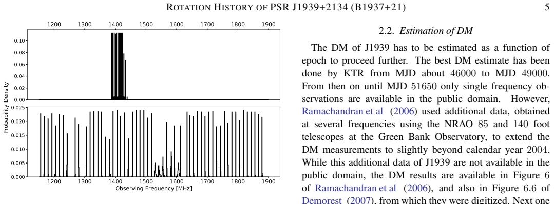
The load-bearing object is the merged, uniformly processed 31-year set of pulse arrival times for J1939. The procedure keeps the entire first public timing data set, prunes the wide-band observations of the second down to a narrow frequency slice around the first data set's frequencies (removing the need for frequency-dependent 'FD' delay parameters), estimates the dispersion measure epoch by epoch with a dual-frequency method and a digitized early DM curve, aligns the 36 instrument sub-systems with fixed clock-offset ('JUMP') terms, and models red-noise (low-frequency wander) correlations using either a spectral function or a power-law harmonic approach in the standard timing-modeling software. The fit that carries the planetary claim is a full Keplerian orbit, with no linearized approximation: the projected semi-major axis $A\approx137$ µs and period $P\approx11{,}300$ days relate through Kepler's third law to a Moon-mass companion at about 11 AU. The competing precession mechanism is the formula $f(t)=k+a_1\sin(\omega_p(t-t_0))-a_2\sin 2(\omega_p(t-t_0))$, whose first and second harmonic amplitudes carry the oblateness and wobble-angle information.

What would settle it

Continue timing J1939 for another ~15–30 years to see whether the sinusoid repeats at the same phase, period, and amplitude; if the residuals do not trace the same curve in the second cycle, both the Moon-mass companion and the precession model are falsified. A shorter-term test is to compute a periodogram of the merged residuals with a red-noise false-alarm threshold: unless the ~31-year peak is significant against that threshold, it should not be assigned to any physical mechanism.

Watch

Extended reading notes

Core claim

The central discovery is that the timing residuals of PSR J1939+2134, after merging the two public long-term timing data sets with one uniform selection and dispersion-measure treatment, are dominated by a near-sinusoidal signal with period $P \approx 11{,}300$ days ($\approx 31$ yr), projected semi-major axis $A \approx 137$ µs, and eccentricity $e \approx 0.21$. A full Keplerian fit gives a companion mass of about $3.5\times 10^{-8}$ solar masses, close to the Moon's mass, in a relative orbit of semi-major axis $\approx 11$ AU. A torque-driven precession model with oblateness $\epsilon \approx 1.6\times 10^{-12}$ and $\theta \tan\chi \approx 0.4$ also fits the data, but with residual scatter about 2.5 times larger than the planetary fit. The paper also reports an unexplained, frequency-independent timing excess of about 8 µs concentrated during the epoch of steepest DM gradient, and a clock-stability level of almost one part in $10^{15}$ over about 31 years.

Load-bearing premise

The load-bearing premise is that the near-sinusoidal ~31-year wobble is a real coherent signal and not a chance realization of slowly wandering timing noise; only one full cycle lies inside the dataset, and the fitted period moves by about two years depending on how the noise is treated.

Editorial extensions

If this is right

If the sinusoid is real, J1939's rotation is a clock stable to almost one part in $10^{15}$ over 31 years, making it one of the most stable celestial clocks known.
A Moon-mass companion at about 11 AU with $e\approx0.2$ would place J1939's planet between the close, nearly circular planets of PSR B1257+12 and the wider, eccentric planet of PSR B0329+54, so any formation scenario must explain both extremes.
If torque-driven precession is instead correct, the inferred oblateness $\epsilon\approx1.6\times10^{-12}$ implies a nearly unstrained, largely decoupled neutron-star crust, consistent with the complete absence of glitches in J1939.
The power-law index $\beta=3.86\pm0.04$ for electron-density fluctuations indicates the interstellar scattering environment along this line of sight has been statistically stable across three decades.
The unexplained ~8 µs excess coinciding with the steepest DM gradient marks a new phenomenon that future multi-frequency monitoring can target directly.

Reading between the lines

Editorial extensions of the paper, not claims the author makes directly.

Because the four fits in the paper give periods spread from 11,105 to 13,068 days, a fair reader should treat the nominal '31-year' period as known only to about ±2 years until a second cycle is observed.
A stronger test would fit a Keplerian companion and a red-noise process simultaneously in one Bayesian model; the paper fits the sinusoid separately from the noise model, so it cannot fully exclude the possibility that the sinusoid is absorbed noise.
If the excess noise during the steepest DM gradient is interstellar, it should appear in other pulsars behind the same scattering screen; if it does not, the excess likely originates in the pulsar's own magnetosphere.
Should the timing baseline reach a second cycle, a stable phase and period would favor the companion, while a drifting period or growing second harmonic would favor torque-driven precession.

Share X Bluesky LinkedIn Reddit HN

Signed reviews

No signed human review yet.

Editorial analysis

A structured set of objections, weighed in public.

Desk editor's note, referee report, and a circularity audit.

Desk Editor's Note

read the letter

You should know two things. First, this is the first analysis to properly combine the IPTA and NANOGrav public data sets for J1939+2134, and the effort put into handling frequency-dependent profile evolution, DM estimation, and inter-sub-system delays is real. Second, the headline result—a moon-mass companion at 11 AU—is not something I would put money on. The paper is honest about its own limits, but those limits are close to the center of the claim.

The genuinely useful parts: a 31-year clock stability estimate at the one-part-in-10^15 level, a clean measurement of the ISM spectral index (beta = 3.86 ± 0.04), a careful DM curve, and a documented excess timing noise episode that coincides with steep DM gradient. These are worth having, and the data-selection scheme for making NANOGrav wide-band data compatible with IPTA narrow-band data is thoughtful. The four-way fits with MCMC error estimation are also more thorough than what the original IPTA or NANOGrav papers did for this pulsar.

The soft spot is the planetary interpretation. The residuals do show a roughly sinusoidal term with a period near the data span, but there is only one cycle in 31 years. The paper's own Table 1 shows the fitted period bouncing between 11105 and 13068 days across four reasonable analyses, a spread of about 2.1 years against formal errors of a few days. The paper acknowledges this and says the larger uncertainty should be used, which is good, but it does not fix the problem. More importantly, there is no formal test against a steep-spectrum red-noise process. The robustness test in Figure 10 excises the first 2–8 years and shows the period drifts from 13068 to 13370 days; the paper reads that as stability, but it is exactly the kind of drift you would expect from a red-noise realization. The reduced chi-square values of 24–39 also tell you the quoted uncertainties are not statistically meaningful under the assumed noise model.

The paper also excludes the MJD 51200–53200 data from the orbit fit because of excess noise whose cause is unknown. That is a significant chunk of the already-short baseline, and it raises the question of what else in the residuals is being absorbed by the model. The precession alternative is presented as a worse fit, which is fair, but neither model is tested against a "no periodic signal" hypothesis.

My take: the paper deserves a serious referee. An editor should not desk-reject it, because the data combination and the timing-noise characterization are useful, and the planet claim, while underdetermined, is not absurd. But the referee should push for a formal likelihood comparison against red-noise-only models, a model of the excluded MJD segment, and a demonstration that the period is stable when fit with a proper noise model. I would cite the DM/clock work, not the planet. And yes, I would bring it to a reading group, mainly to argue about the red-noise analysis.

Referee Report

4 major / 5 minor

Summary. The manuscript presents a uniform reanalysis of 31 years of public IPTA and NANOGrav timing data for the millisecond pulsar PSR J1939+2134 (B1937+21). It derives a dispersion-measure curve, applies consistent data selection and instrumental-offset corrections across 36 sub-systems, and models red-noise correlations with both the IPTA and NANOGrav prescriptions. The resulting timing residuals are reported to be very close to a sinusoid with period about 31 years. The paper fits this timing noise with a Keplerian planetary-companion model, obtaining a projected semi-major axis A of about 137 microseconds, eccentricity e about 0.215, and period P about 11296 days, which it interprets as a Moon-sized companion at about 11 AU; a precession model is fitted as an alternative. Additional results include a clock stability of almost one part in 10^15, an interstellar electron-density spectral index beta = 3.86 +/- 0.04, and excess achromatic timing noise of about 8 microseconds amplitude during epochs of steep DM gradient.

Significance. If the quasi-sinusoidal timing residual is a coherent, deterministic signal, then the paper reports a notable result for millisecond-pulsar timing and for planet formation around recycled pulsars. The manuscript has real strengths: the careful merging of heterogeneous public data, the explicit handling of 36 instrumental sub-systems, the cross-check between two independent red-noise treatments, and the candid reporting of large reduced chi-square values and the one-cycle limitation. However, the central claim that the timing noise is a true periodicity rather than a realization of steep-spectrum red noise is not yet supported by a model comparison, and the fitted period is not robust across the four analyses. The significance of the paper is therefore conditional: the data combination and the descriptive fits are valuable, but the companion and precession interpretations require substantially stronger statistical evidence.

major comments (4)

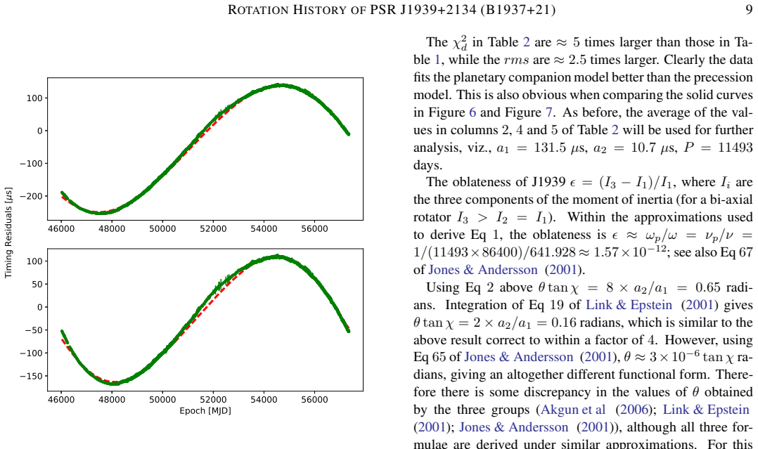
[Section 3.2, Figures 6 and 7] The paper fits deterministic sinusoidal (Keplerian and precession) models to the timing residuals but never compares them against a red-noise-only model, such as a power-law or harmonic process with the same white-noise and T2 treatment. With only one cycle of the putative 31-year period in the data, a realization of steep-spectrum red noise can plausibly produce the same apparent curvature. A likelihood ratio, Bayes factor, or false-alarm probability against a red-noise-only process is needed before the claim that the timing noise is 'very close to a sinusoid' can be accepted.
[Section 3.2.1, Table 1 and Section 5.2] The orbital period is not robust: the four analyses give P = 11105, 13068, 11403, and 11381 days, a spread of about 2.1 years against formal errors of a few days. The paper itself acknowledges this in Section 5.2 and advises using the larger uncertainty, but the companion mass of about 3.5 x 10^-8 solar masses is quoted without propagating this systematic period uncertainty. The derived companion mass and semi-major axis are therefore not established to the accuracy implied by the text.
[Section 3.2.1, Figure 6 and Section 3.3] The fit explicitly ignores the excess timing noise between MJD 51200 and 53200, which spans about 5.5 years of the 31-year baseline. Excluding a large contiguous block of data from a fit to a long-period sinusoid can bias the estimated period and amplitude, especially when the excluded interval coincides with a large DM-gradient epoch. The paper should either model this excess noise simultaneously, include it with an additional variance term, or demonstrate explicitly that its exclusion does not change the inferred period and amplitude beyond the quoted uncertainties.
[Section 3.2.2, Tables 1 and 2] The preference for the planetary-companion model over the precession model is based on the rms and reduced chi-square of the best fits, but the reduced chi-square values in both tables are 24-39 and 104-226 respectively, far above unity. This indicates that the formal parameter uncertainties are not statistically meaningful under the assumed noise model, so the comparison of the two models is not a valid model selection without a common treatment of the noise and a proper goodness-of-fit or Bayesian evidence calculation.

minor comments (5)

[Equation (1)] The notation 'sin 2 (omega_p (t - t_0))' in Equation (1) is ambiguous: it should be written as sin(2 omega_p (t - t_0)) or with an explicit square, as the context indicates a second harmonic rather than a squared sine.
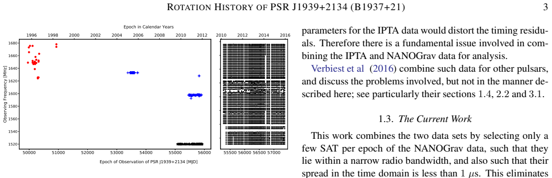
[Figures 1, 2, and 5] Several axis labels contain corrupted characters, for example 'T m ng Res duals' and 'Calenda( Yea(' in Figure 1, and 'Epoch in Calenda( Yea(' in Figure 5. These should be fixed in the final version.
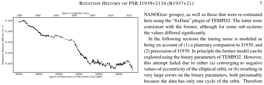
[Section 3.1] The value beta = 3.86 +/- 0.04 is derived from a spline fit to the DM data, but the spline smoothing and the absence of error bars on the earlier digitized DM points are not fully propagated into this uncertainty. The quoted error likely underestimates the systematic contribution from the spline model choice.
[Section 5.2, Table 4] The statement that there is 'no correlation' of the derived period with the length of data used is not quantitatively supported. Table 4 shows P increasing monotonically from 13068 to 13370 days as the first 0 to 8 years are excised; a correlation coefficient or a significance test should be reported.
[Section 2.2] The digitized DM curve from Ramachandran et al. (2006) and Demorest (2007) is used without a description of the digitization uncertainty beyond the alignment rms of 3 x 10^-4 pc cm^-3. A brief discussion of how the digitization error enters the DM curve and the subsequent timing analysis would improve reproducibility.

Circularity Check

0 steps flagged · score 0.0 of 10

No significant circularity: the planet/precession parameters are fit to the timing residuals and the derived masses follow from standard formulas; the main caveats are model-comparison issues, not circular logic.

full rationale

The paper's derivation chain is self-contained in the sense that no claimed result is equivalent to its own input by construction. The timing residuals are produced by standard TEMPO2 timing fits to the combined public IPTA and NANOGrav data. The sinusoidal timing noise is then fit independently by a full Keplerian planetary model and by a precession model, and the quoted companion mass and oblateness are computed from the fitted amplitudes and periods using standard Keplerian and precession formulae. The apparent self-citation to Vivekanand (2017) for Eq. 2 is not load-bearing: the formula is the standard Keplerian mass function, and the paper's central claims do not rest on an unverified self-cited theorem. The paper explicitly acknowledges the key limitations: only one orbital/precession cycle is in the data, the fitted periods scatter by about 2.1 years across the four analyses, and the reduced chi-square values are large. Those are statistical and model-comparison concerns about whether a red-noise-only process could mimic the quasi-sinusoid, but they are not circularity. The clock-stability statement is conditional on the adopted timing-noise model and represents a model-subtraction interpretation rather than a derivation that assumes its own conclusion. No step in the paper reduces a prediction to a fitted input or imports a uniqueness claim from the authors' prior work.

Assumptions & free parameters 7 free parameters · 5 assumptions · 1 invented entities

The analysis is honest about its inputs: 35 instrumental JUMP offsets, per-subsystem T2EFAC and T2EQUAD values, and the DM spline are fitted or adopted, and the red-noise model parameters come from earlier IPTA and NANOGrav analyses. The central planet and precession interpretations depend on the unproven coherence of a single-cycle 31-year sinusoid and on the assumption that selecting narrowband SATs removes all frequency-evolution systematics. No new entity with independent evidence is introduced beyond the inferred companion.

free parameters (7)

Planetary orbit parameters (A, e, P, T0, omega) = Fitted A, e, P values are about 137.2 microseconds, 0.215, and 11296 days.
These are fit to the timing noise in Section 3.2.1; the moon mass is derived from A and P through Eq. 2 of Vivekanand (2017).
Precession model parameters (a1, a2, P) = Fitted a1, a2, P values are about 131.5 microseconds, 10.7 microseconds, and 11493 days.
These are fit to the timing noise in Section 3.2.2, and the oblateness and wobble angle are derived from them.
DM spline model = The spline fit has an RMS residual of about 3e-4 pc cm^-3.
The spline in Figure 5 is fit to the DM data and is used instead of raw DM data to compute the phase structure function and the spectral index beta.
ISM turbulence spectral index beta = Fitted value is 3.86 with a formal uncertainty of 0.04.
This is the slope of the phase structure function and is one of the paper's headline results.
Instrumental JUMP offsets for 36 subsystems = Fitted offsets are listed in Figure 3 and range from about -747.8 to +175.5 microseconds.
These are estimated to align data from different telescopes and are held fixed in TEMPO2, so the timing residuals depend on them.
T2EFAC and T2EQUAD per subsystem = Values are re-estimated locally with the fixData plugin and differ from the original values for some subsystems.
These parameters scale and inflate the uncertainties, and they affect the reduced chi-square and the formal errors on the orbit.
IPTA red-noise covariance parameters (alpha, fc, a) = Values used include alpha 3.016 or 5.098, fc 0.0322, and a 6.4e-23 or 9.8e-20.
These parameters describe the red-noise correlation model used by the IPTA method and are obtained from the data via autoSpectralFit.

assumptions (5)

domain assumption The selected narrow subset of NANOGrav data has negligible pulse-profile frequency evolution, so FD parameters are not needed.
Section 2.1 builds the data-combination strategy on this; if it is wrong, the aligned SATs carry frequency-dependent systematics.
domain assumption The apparent ~31-year sinusoid is coherent timing noise rather than a red-noise realization.
Sections 3.2 and 4; P is close to the data span and varies by about 2 years across fits, so this assumption is load-bearing for both models.
domain assumption The spline fit to the DM is a faithful representation of the true DM variations and can be used to compute the phase structure function.
Section 3.1; the raw DM data cannot be used directly because the earlier half lacks error bars.
domain assumption The IPTA and NANOGrav red-noise correlation models adequately describe the low-frequency noise of J1939.
Section 2.3 and Table 1; the derived period and its uncertainty depend on which red-noise model is used.
domain assumption Keplerian orbital motion and the precession equations from Akgun et al. (2006), Link and Epstein (2001), and Jones and Andersson (2001) apply to J1939.
Equations 1 and 2 and Section 3.2.2; if the precession model is wrong, the derived oblateness and wobble angle are invalid.

invented entities (1)

Moon-sized planetary companion around PSR J1939+2134
purpose: To explain the ~31-year sinusoidal timing residuals via a Keplerian orbit at about 11 AU with eccentricity near 0.21.
The orbit parameters are fit to the same timing residuals used to claim the planet; there is no independent detection, and the paper itself notes that only one orbit cycle is available.

how reviews work

0 comments

Cite this review

Pith. "Pith review of The 31-year Rotation History of the Millisecond Pulsar J1939+2134 (B1937+21)." pith.science (2026). https://pith.science/paper/LILTGZX3

@misc{pith2026190803026,
  author       = {Pith},
  title        = {Pith review of: The 31-year Rotation History of the Millisecond Pulsar J1939+2134 (B1937+21)},
  year         = {2026},
  howpublished = {\url{https://pith.science/paper/LILTGZX3}},
  note         = {Machine review of arXiv:1908.03026}
}

abstract

The timing properties of the millisecond pulsar PSR J1939+2134 -- very high rotation frequency, very low time derivative of rotation frequency, no timing glitches and relatively low timing noise -- are responsible for its exceptional timing stability over decades. It has been timed by various groups since its discovery, at diverse radio frequencies, using different hardware and analysis methods. Most of this timing data is now available in the public domain in two segments, which have not been combined so far. This work analyzes the combined data by deriving uniform methods of data selection, derivation of Dispersion Measure (DM), accounting for correlation due to "red" noise, etc. The timing noise of this pulsar is very close to a sinusoid, with a period of approximately $31$ years. The main results of this work are (1) The clock of PSR J1939+2134 is stable at the level of almost one part in $10^{15}$ over about $31$ years, (2) the power law index of the spectrum of electron density fluctuations in the direction of PSR J1939+2134 is $3.86 \pm 0.04$, (3) a Moon sized planetary companion, in an orbit of semi major axis about $11$ astronomical units and eccentricity $\approx 0.2$, can explain the timing noise of PSR J1939+2134, (4) Precession under electromagnetic torque with very small values of oblateness and wobble angle can also be the explanation, but with reduced confidence, and (5) there is excess timing noise of about $8$ $\mu$s amplitude during the epochs of steepest DM gradient, of unknown cause.

Figures

Figures reproduced from arXiv: 1908.03026 by the authors.

**Figure 1.** 31 years of timing residuals of J1939 along with error bars, after removal of timing noise, which is estimated by TEMPO2 using 100 noise harmonics, as explained later in the text. Timing Array (PPTA) data. Due to instrumentation and methodology differences, the earlier ≈ 8 years of the data from the North American radio observatories are combined with the EPTA and PPTA data to form what is known as the International… view at source ↗

**Figure 2.** Illustration of incompatibility between IPTA and NANOGrav data, using the 1600 MHz L-band data. The left panel plots the radio frequency of observation of the IPTA data from Parkes (dots), Jodrell Bank (+) and Nancay (*) Observatories. The right panel displays the NANOGrav data from the Green Bank Observatory that corresponds to the same frequency range as that in the left panel, although the actual frequency range… view at source ↗

**Figure 3.** Summary of IPTA and NANOGrav observations of J1939 that are available in the public domain. The first column of labels of the left ordinate are: (1) AR = Arecibo Telescope, (2) EFF = Effelsberg Telescope, (3) GBT = Green Bank Telescope, (4) JBO = Jodrell Bank Observatory, (5) NRT = Nancay Radio Telescope, (6) PKS = Parkes Telescope, and (7) WSRT = Westerbork Synthesis Radio Telescope. The second column of labels ar… view at source ↗

Figures from the paper (6 more)

**Figure 4.** Figure 4: Probability distribution of frequency of observation for the Rcvr1 2 GASP (top panel) and Rcvr1 2 GUPPI (bottom panel) sub-systems, respectively. statistically significant SAT. This scheme will probably not work with wide band data from smaller radio telescopes. The da…

**Figure 5.** Figure 5: DM of J1939 as a function of epoch for the combined IPTA and NANOGrav data. The earlier DMs have a fixed error of 3 × 10−4 pc cm−3 , which is explained in the text; the later DMs have estimated errors. The dashed line is a spline curve that best fits the data. The maxi…

**Figure 6.** Figure 6: The data in the two panels were obtained using the IPTA (top panel) and the NANOGrav (bottom panel) methods of correction for “red” noise correlation; in both cases re-estimated T2 parameters were used. The dashed line in each panel represents the best fit planetary …

**Figure 7.** Figure 7: The data is the same as in [PITH_FULL_IMAGE:figures/full_fig_p009_7.png]

**Figure 8.** Figure 8: Difference between the data and the modeled curves of [PITH_FULL_IMAGE:figures/full_fig_p012_8.png]

**Figure 10.** Figure 10: Difference between the data and the modeled curves of top panel of [PITH_FULL_IMAGE:figures/full_fig_p013_10.png]

Discussion (0). Continue with ORCID to comment.

Reference graph

Works this paper leans on

35 extracted references · 34 canonical work pages

[1]

2006, MNRAS, 365, 653

Akgun, T., Link B., & Wasserman I . 2006, MNRAS, 365, 653

work page 2006
[2]

& Shaham, J

Alpar, M.A., Anderson, P .W., Pines, D. & Shaham, J. 1984, ApJ, 276, 325

work page 1984
[3]

2014, ApJ, 794, 141

Arzoumanian, Z., Brazier, A., Burke-Spolaor, S. 2014, ApJ, 794, 141

work page 2014
[4]

2015, ApJ, 813, 65

Arzoumanian, Z., Brazier, A., Burke-Spolaor, S. 2015, ApJ, 813, 65

work page 2015
[5]

2018, ApJS , 235, 37 Backer D.C., Kulkarni S.R., Heiles C., Davis M.M., Goss W.M

Arzoumanian, Z., Brazier, A., Burke-Spolaor, S. 2018, ApJS , 235, 37 Backer D.C., Kulkarni S.R., Heiles C., Davis M.M., Goss W.M. , 1982, Nature, 300, 615

work page 2018
[6]

Backer, D. C. and Hellings, R. W. 1986, ARA&A, 24, 537

work page 1986
[7]

Buchner, J., Georgakakis, A., Nandra, K., et al 2014, A&A, 56 4, A125

work page 2014
[8]

et al 2016, MNRAS, 45 7, 4421

Caballero, R.N., Lee, K.J., Lentati, L. et al 2016, MNRAS, 45 7, 4421

work page 2016

Show all 35 references

[9]

Hobbs, G., Champion, D.J., Manchester, R.N., & J

Coles, W,. Hobbs, G., Champion, D.J., Manchester, R.N., & J. P . W. V erbiest, J.P .W. 2011, MNRAS, 418, 561 Cordes J.M., Wolszczan A., Dewey R.J., Blaskiewicz M., Stinebring D.R., 1990, ApJ, 349, 245

2011
[10]

2007, Ph

Demorest, P .B. 2007, Ph. D. Thesis, Univ. of California, Berkeley

2007
[11]

B., and Manchester, R

Edwards, R.T., Hobbs, G. B., and Manchester, R. N. 2006, MNRAS, 372, 1549

2006
[12]

2018, Front iers of

Feigelson, E.D., Jogesh Babu, G., Caceres, G.A. 2018, Front iers of

2018
[13]

2008, MNRAS, 384, 449 Feroz F., Hobson M.P ., Bridges M

Physics, Article 80 Feroz F., Hobson M.P . 2008, MNRAS, 384, 449 Feroz F., Hobson M.P ., Bridges M. 2009, MNRAS, 398, 1601

2008
[14]

B., Edwards, R.T

Hobbs, G. B., Edwards, R.T. and Manchester, R. N. 2006, MNRAS, 369, 655

2006
[15]

2010, arXiv:1008.4686

Hogg, D.W., Bovy, J., Lang, D. 2010, arXiv:1008.4686

2010 arXiv
[16]

2012, arXiv:1205.4446

Hogg, D.W. 2012, arXiv:1205.4446

2012 arXiv
[17]

2017, ApJS, 236, 11 Hotan A.W., Bailes M., Ord S.M., 2006, MNRAS, 369, 1502

Hogg, D.W., Foreman-Mackey, D. 2017, ApJS, 236, 11 Hotan A.W., Bailes M., Ord S.M., 2006, MNRAS, 369, 1502

2017
[18]

2001, MNRAS, 324, 811

Jones, D.I., Andersson, N. 2001, MNRAS, 324, 811

2001
[19]

et al 2001, SciPy: Open Source Scientiﬁc Tools for Python

Jones, E., Oliphant, E., Peterson, P . et al 2001, SciPy: Open Source Scientiﬁc Tools for Python

2001
[20]

& Ryba, M.F

Kaspi, V .M., Taylor, J.H. & Ryba, M.F. 1994, ApJ, 428, 713 (KTR)

1994
[21]

2015, Ap J, 801, 130

Lam, M.T., Cordes, J.M., Chatterjee, S., & Dolch, T. 2015, Ap J, 801, 130

2015
[22]

et al 2014, MNRAS, 437, 3004

Lentati, L., Alexander, P ., Hobson, M.P . et al 2014, MNRAS, 437, 3004

2014
[23]

et al 2015, MN RAS, 435, 2576

Lentati, L., Taylor, S.R., Mingarelli, C.M.F. et al 2015, MN RAS, 435, 2576

2015
[24]

2001, ApJ, 556, 392

Link, B., Epstein, R.I. 2001, ApJ, 556, 392

2001
[25]

G., and Graham Smith, F

Lyne, A. G., and Graham Smith, F. 2006, Pulsar Astronomy, Cambridge Astrophysics

2006
[26]

Planets Around Pulsars

Malhotra, R., in “Planets Around Pulsars”, ASP Conference S eries, V ol 36, pp 89, 1993, Eds J.A. Philips, J.E. Thorsett and S.R. Kulkarni

1993
[27]

Manchester, R. N. and Taylor, J. H. 1977, Pulsars, W. H. Freem an Manchester R.N., Hobbs G., Bailes M. et al 2013, Publ. Astron . Soc. Aust., 30, 17

1977
[28]

& Thorsett, S.E

Phillips, J.A. & Thorsett, S.E. 1994, Astrophysics and Spac e Science, 212, 91

1994
[29]

Ramachandran, R., Demorest, P ., Backer, D.C., et al 2006, ApJ, 645, 303

2006
[30]

1977, ApJ, 214, 251

Shaham, J. 1977, ApJ, 214, 251

1977
[31]

2010, ApJ, 725, 1607

Shannon, R.M., Cordes, J.M. 2010, ApJ, 725, 1607

2010
[32]

et al 2013, ApJ, 766, 5

Shannon, R.M., Cordes, J.M., Metcalfe, T.S. et al 2013, ApJ, 766, 5

2013
[33]

& Rodin, A.E

Starovoit, E.D. & Rodin, A.E. 2017, Astronomy Reports, 61, 9 48 van Haasteren, R. & V allisneri, M. 2014, PHYSICAL REVIEW D 90, 104012 V erbiest, J.P .W., Bailes, M., Coles, W.A., et al 2009, MNRAS, 400, 951 V erbiest, J.P .W., Lentati, L., Hobbs, G., et al 2016, MNRAS,458, 1267

2017
[34]

2017, arXiv:1710.05293

Vivekanand, M. 2017, arXiv:1710.05293

2017 arXiv
[35]

& Frail, D.A

Wolszczan, A. & Frail, D.A. 1992, Nature, 355, 145 Y ou, X.P ., Hobbs, G., Coles, W.A., et al 2007, MNRAS, 378, 493

1992

Pith tools

Reviewed August 14, 2026 · model on record in the stance chip above.

[1] [1]

2006, MNRAS, 365, 653

Akgun, T., Link B., & Wasserman I . 2006, MNRAS, 365, 653

work page 2006

[2] [2]

& Shaham, J

Alpar, M.A., Anderson, P .W., Pines, D. & Shaham, J. 1984, ApJ, 276, 325

work page 1984

[3] [3]

2014, ApJ, 794, 141

Arzoumanian, Z., Brazier, A., Burke-Spolaor, S. 2014, ApJ, 794, 141

work page 2014

[4] [4]

2015, ApJ, 813, 65

Arzoumanian, Z., Brazier, A., Burke-Spolaor, S. 2015, ApJ, 813, 65

work page 2015

[5] [5]

2018, ApJS , 235, 37 Backer D.C., Kulkarni S.R., Heiles C., Davis M.M., Goss W.M

Arzoumanian, Z., Brazier, A., Burke-Spolaor, S. 2018, ApJS , 235, 37 Backer D.C., Kulkarni S.R., Heiles C., Davis M.M., Goss W.M. , 1982, Nature, 300, 615

work page 2018

[6] [6]

Backer, D. C. and Hellings, R. W. 1986, ARA&A, 24, 537

work page 1986

[7] [7]

Buchner, J., Georgakakis, A., Nandra, K., et al 2014, A&A, 56 4, A125

work page 2014

[8] [8]

et al 2016, MNRAS, 45 7, 4421

Caballero, R.N., Lee, K.J., Lentati, L. et al 2016, MNRAS, 45 7, 4421

work page 2016